![]()
![]()
xpose was designed as a ggplot2-based alternative to xpose4. xpose aims to reduce the post processing burden and improve diagnostics commonly associated the development of non-linear mixed effect models.
# Install the lastest release from the CRAN
install.packages('xpose')

# Or install the development version from GitHub
# install.packages('devtools')
devtools::install_github('UUPharmacometrics/xpose')library(xpose)xpdb <- xpose_data(runno = '001')xpdbrun001.lst overview:
- Software: nonmem 7.3.0
- Attached files (memory usage 1.4 Mb):
+ obs tabs: $prob no.1: catab001.csv, cotab001, patab001, sdtab001
+ sim tabs: $prob no.2: simtab001.zip
+ output files: run001.cor, run001.cov, run001.ext, run001.grd, run001.phi, run001.shk
+ special: <none>
- gg_theme: theme_readable
- xp_theme: theme_xp_default
- Options: dir = data, quiet = TRUE, manual_import = NULLsummary(xpdb, problem = 1)Summary for problem no. 0 [Global information]
- Software @software : nonmem
- Software version @version : 7.3.0
- Run directory @dir : data
- Run file @file : run001.lst
- Run number @run : run001
- Reference model @ref : 000
- Run description @descr : NONMEM PK example for xpose
- Run start time @timestart : Mon Oct 16 13:34:28 CEST 2017
- Run stop time @timestop : Mon Oct 16 13:34:35 CEST 2017
Summary for problem no. 1 [Parameter estimation]
- Input data @data : ../../mx19_2.csv
- Number of individuals @nind : 74
- Number of observations @nobs : 476
- ADVAN @subroutine : 2
- Estimation method @method : foce-i
- Termination message @term : MINIMIZATION SUCCESSFUL
- Estimation runtime @runtime : 00:00:02
- Objective function value @ofv : -1403.905
- Number of significant digits @nsig : 3.3
- Covariance step runtime @covtime : 00:00:03
- Condition number @condn : 21.5
- Eta shrinkage @etashk : 9.3 [1], 28.7 [2], 23.7 [3]
- Epsilon shrinkage @epsshk : 14.9 [1]
- Run warnings @warnings : (WARNING 2) NM-TRAN INFERS THAT THE DATA ARE POPULATION.
Summary for problem no. 2 [Model simulations]
- Input data @data : ../../mx19_2.csv
- Number of individuals @nind : 74
- Number of observations @nobs : 476
- Estimation method @method : sim
- Number of simulations @nsim : 20
- Simulation seed @simseed : 221287
- Run warnings @warnings : (WARNING 2) NM-TRAN INFERS THAT THE DATA ARE POPULATION.
(WARNING 22) WITH $MSFI AND "SUBPROBS", "TRUE=FINAL" ...dv_vs_ipred(xpdb)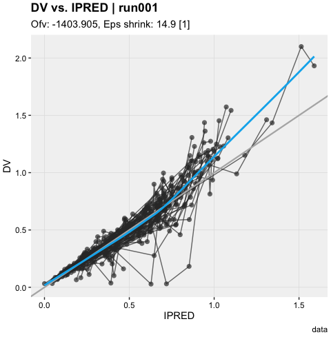
ind_plots(xpdb, page = 1)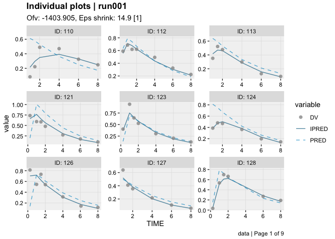
xpdb %>%
  vpc_data(stratify = 'SEX', opt = vpc_opt(n_bins = 7, lloq = 0.1)) %>%
  vpc()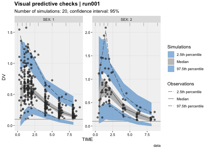
eta_distrib(xpdb, labeller = 'label_value')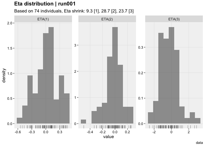
prm_vs_iteration(xpdb, labeller = 'label_value')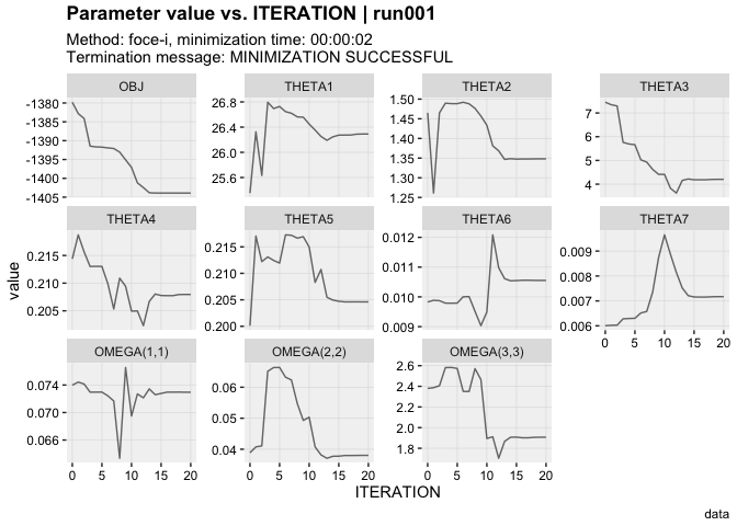
The xpose website contains several useful articles to make full use of xpose
When working with xpose, a working knowledge of ggplot2 is recommended. Help for ggplot2 can be found in:
Please note that the xpose project is released with a Contributor Code of Conduct and Contributing Guidelines. By contributing to this project, you agree to abide these.