xplaineff: Regional Feature Effects for Better Model Explanations

The xplaineff R package implements the GADGET algorithm for interpretable machine learning. It recursively partitions the feature space to minimize the heterogeneity of feature effects (e.g., Accumulated Local Effects or Partial Dependence), producing a tree of regions where effects are more stable and easier to interpret. The package integrates with the mlr3 ecosystem.

Features

• Interaction detection: Identifies feature interactions by recursively splitting on heterogeneity of effects.
• ALE and PD support: AleStrategy for ALE (computed internally from a model), and PdStrategy for PD/ICE (via precomputed effects or internal computation from a model).
• Visualization: Tree structure plots and regional effect curves (ALE, PD, ICE).
• Extensible design: R6-based strategy pattern; plug in custom effect strategies.
• Performance: Core calculations in C++ (Rcpp/RcppArmadillo).

Installation

Install the development version from GitHub:

# install.packages("devtools")
devtools::install_github("mlr-org/xplaineff")

Requires R6, ggplot2, data.table, Rcpp; see DESCRIPTION for details. The examples below additionally use:

install.packages(c("mlr3", "mlr3learners", "ranger", "ISLR2"))

API overview

Fit arguments

• AleStrategy-specific
  • model (required): fitted mlr3 learner used to compute ALE.
  • effect (reserved): currently not enabled; reserved for future extension.
  • n_intervals (optional): number of intervals for ALE grids (default: 10).
  • predict_fun (optional): custom prediction function; if NULL, uses the learner’s default.
  • order_method (optional): how to order categorical split-feature levels before searching over binary splits. Internally, GADGET builds a pairwise distance matrix between levels (using other features), embeds it into 1D, and searches ordered-prefix partitions. The learned order is only used to define candidate partitions; plots display category sets rather than implying a semantic ordering. Supported methods are:
    • "raw" (default): keep the original factor level order (no reordering).
    • "mds": multi-dimensional scaling on the level-distance matrix, then order levels by the 1D coordinates.
    • "pca": PCA on the level-distance matrix, then order levels by the first principal component.
    • "random": use a random order of levels (mainly for robustness checks or baselines).
• PdStrategy-specific
  • effect (optional): object of class FeatureEffects (e.g. from iml::FeatureEffects).
  • model (optional): fitted model used for internal PD/ICE computation when effect is not provided.
  • n_grid (optional): number of grid points for numeric PD/ICE computation (default: 20).
  • predict_fun (optional): custom prediction function for internal PD/ICE computation.
• Shared tree arguments (both strategies)
  • feature_set (optional): subset of features used to compute and plot effects.
  • split_feature (optional): subset of features allowed as splitting variables.
  • impr_par: minimum required improvement in heterogeneity to accept a split.
  • min_node_size: minimum number of observations in each node.
  • n_quantiles: number of candidate split points per numerical feature.

Methodology

GADGET recursively partitions the feature space. At each node it:

1. Computes effect heterogeneity (e.g., variance of ALE derivatives or PD/ICE curves).
2. Searches for a split (on a chosen feature) that maximally reduces heterogeneity.
3. Splits if the reduction exceeds a threshold (impr_par) and node size is sufficient.

Splits isolate regions where feature effects are more stable, revealing interaction structure.

Quick Start

This section shows how to use GADGET with PD and ALE on the Bikeshare data. We first build a PD-based tree with internally computed effects, then an ALE-based tree with internally computed effects.

PD + Bikeshare

library(xplaineff)
library(mlr3)
library(mlr3learners)
library(ISLR2)

# 1) Load and subsample the Bikeshare data
data("Bikeshare", package = "ISLR2")
set.seed(123)
bike = Bikeshare[sample(seq_len(nrow(Bikeshare)), 1000), ]
bike$workingday = as.factor(bike$workingday)
bike_data = bike[, c("hr", "temp", "workingday", "bikers")]
names(bike_data)[names(bike_data) == "bikers"] = "target"

# 2) Fit a black-box regression model with mlr3
task = TaskRegr$new(id = "bike", backend = bike_data, target = "target")
learner = lrn("regr.ranger")
learner$train(task)

# 3) Grow a PD-based GadgetTree on top of the model
tree = GadgetTree$new(
  strategy = PdStrategy$new(),
  n_split = 2,
  min_node_size = 50
)
tree$fit(
  data = bike_data,
  target_feature_name = "target",
  model = learner,
  n_grid = 20L
)

# 4) Inspect the tree structure, splits, and regional PD/ICE curves
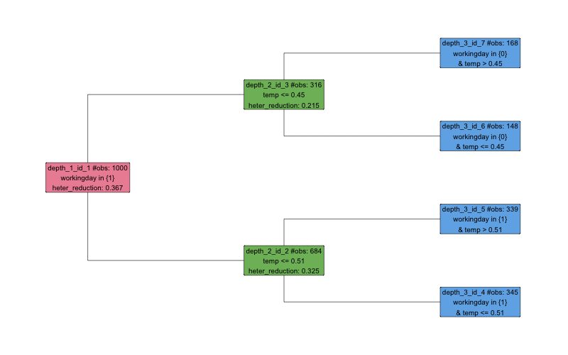
tree$plot_tree_structure()
tree$extract_split_info()
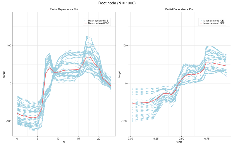
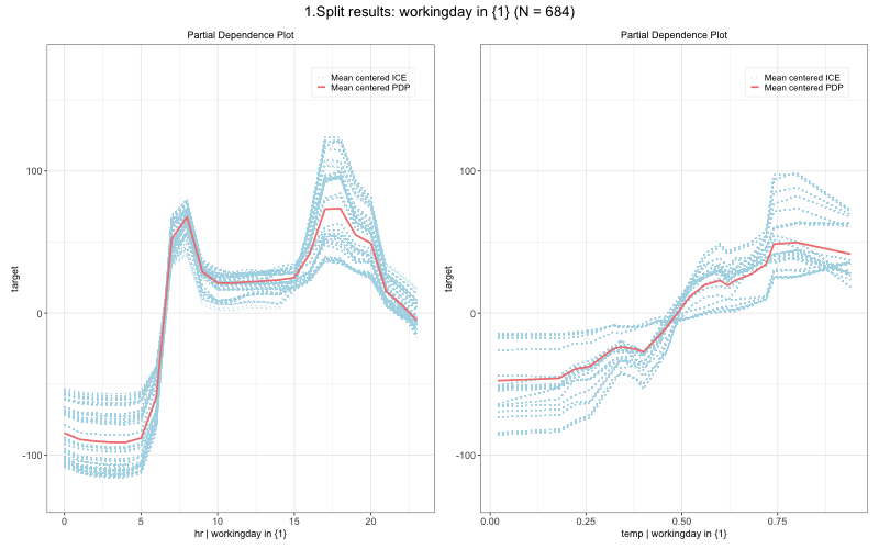
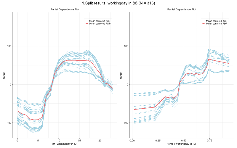
tree$plot(
  data = bike_data,
  target_feature_name = "target",
  features = c("hr", "temp")
)

Pre-computed ICE/PD effects (e.g. from iml::FeatureEffects) can be passed via tree$fit(effect = effect, ...) instead of model =.

Sample split info (PD + Bikeshare):

Tree structure and regional PD/ICE plots (root and first split):

ALE + Bikeshare

library(xplaineff)
library(mlr3)
library(mlr3learners)
library(ISLR2)

# 1) Load and subsample the Bikeshare data
data("Bikeshare", package = "ISLR2")
set.seed(123)
bike = Bikeshare[sample(seq_len(nrow(Bikeshare)), 1000), ]
bike$workingday = as.factor(bike$workingday)
bike_data = bike[, c("hr", "temp", "workingday", "bikers")]
names(bike_data)[names(bike_data) == "bikers"] = "target"

# 2) Fit a black-box regression model with mlr3
task = TaskRegr$new(id = "bike", backend = bike_data, target = "target")
learner = lrn("regr.ranger")
learner$train(task)

# 3) Grow an ALE-based GadgetTree on top of the model
tree = GadgetTree$new(
  strategy = AleStrategy$new(),
  n_split = 2,
  impr_par = 0.01,
  min_node_size = 50
)
tree$fit(
  data = bike_data,
  target_feature_name = "target",
  model = learner,
  n_intervals = 10
)

# 4) Inspect the tree structure, splits, and regional ALE plots
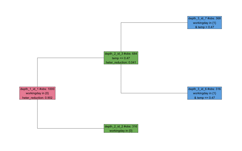
tree$plot_tree_structure()  # prints the tree topology (depth, node IDs, split features)
tree$extract_split_info()
tree$plot(
  data = bike_data,
  target_feature_name = "target",
  features = c("hr", "temp"),
  mean_center = TRUE
)

Sample split info (ALE + Bikeshare):

Tree structure and regional ALE plots (root and first split):

More plot options

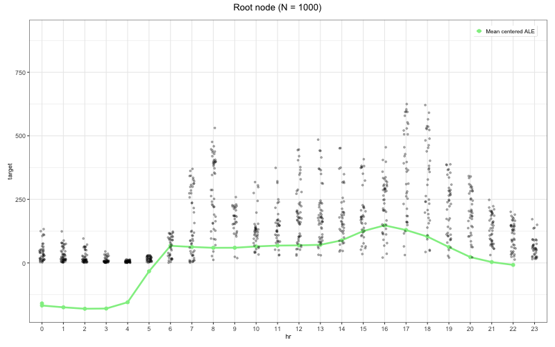
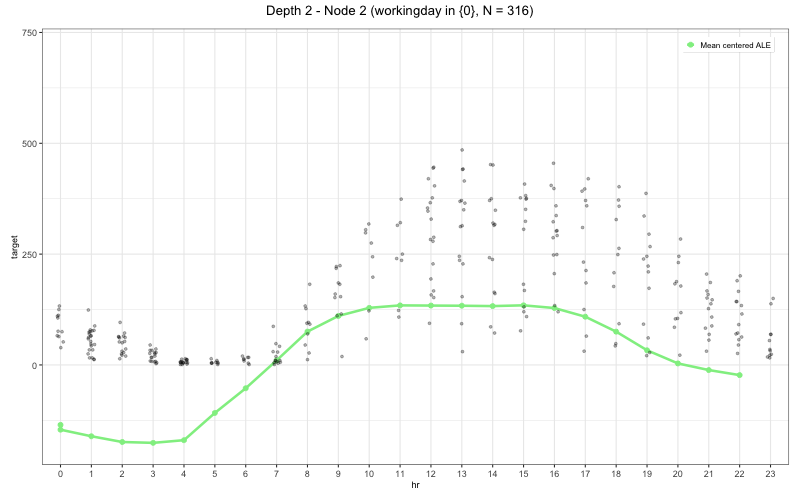
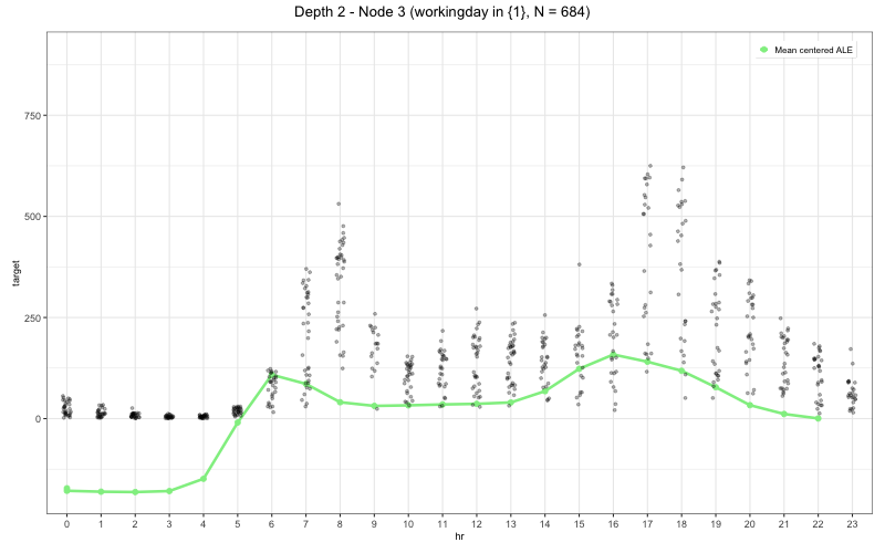
The tree$plot() method is flexible and can be used to drill down into specific depths, nodes, and features. It always returns a nested list of plot objects named by depth and by the actual tree node id, for example pl$Depth_2$Node_3.

• Controlling which nodes to plot

  # Only depth 1 (root)
  pl = tree$plot(
    data = bike_data,
    target_feature_name = "target",
    features = c("hr", "temp"),
    depth = 1
  )
  
  # A specific node at depth 2 (e.g., right child)
  pl = tree$plot(
    data = bike_data,
    target_feature_name = "target",
    features = c("hr", "temp"),
    depth = 2,
    node_id = 3  # see node IDs in tree$plot_tree_structure()
  )
  
  # Inspect or manually print a single plot object
  print(pl$Depth_2$Node_3)

• Selecting features and centering

  # Only plot effects for "hr", without mean-centering
  pl = tree$plot(
    data = bike_data,
    target_feature_name = "target",
    features = "hr",
    mean_center = FALSE
  )

• Overlaying raw observations

  If available for your strategy, you can overlay observed ((x, y)) points on top of the regional curves:

  pl = tree$plot(
    data = bike_data,
    target_feature_name = "target",
    features = c("hr", "temp"),
    mean_center = TRUE,
    show_point = TRUE  # add raw data points
  )

In practice, a common workflow is:

1. Use tree$plot_tree_structure() and tree$extract_split_info() to identify interesting regions.
2. Call tree$plot() with depth / node_id / features to inspect those regions.
3. Manually inspect or save individual plots with named entries such as print(pl$Depth_2$Node_3).

Documentation

• In R: ?xplaineff, ?GadgetTree, ?AleStrategy, ?PdStrategy

Citation

Herbinger, J., Wright, M. N., Nagler, T., Bischl, B., and Casalicchio, G. (2024). Decomposing Global Feature Effects Based on Feature Interactions. Journal of Machine Learning Research, 25(23-0699), 1–65. https://jmlr.org/papers/volume25/23-0699/23-0699.pdf

License

MIT