![]()
![]()
![]()
![]()
The goal of workflowsets is to allow users to create and easily fit a large number of models. workflowsets can create a workflow set that holds multiple workflow objects. These objects can be created by crossing all combinations of preprocessors (e.g., formula, recipe, etc) and model specifications. This set can be tuned or resampled using a set of specific functions.
You can install the released version of workflowsets from CRAN with:
install.packages("workflowsets")And the development version from GitHub with:
install.packages("pak")
pak::pak("tidymodels/workflowsets")Sometimes it is a good idea to try different types of models and preprocessing methods on a specific data set. The tidymodels framework provides tools for this purpose: recipes for preprocessing/feature engineering and parsnip model specifications. The workflowsets package has functions for creating and evaluating combinations of these modeling elements.
For example, the Chicago train ridership data has many numeric predictors that are highly correlated. There are a few approaches to compensating for this issue during modeling:
Use a feature filter to remove redundant predictors.
Apply principal component analysis to decorrelate the data.
Use a regularized model to make the estimation process insensitive to correlated predictors.
The first two methods can be used with any model while the last option is only available for specific models. Let’s create a basic recipe that we will build on:
library(tidymodels)
data(Chicago)
# Use a small sample to keep file sizes down:
Chicago <- Chicago |> slice(1:365)

base_recipe <-
  recipe(ridership ~ ., data = Chicago) |>
  # create date features
  step_date(date) |>
  step_holiday(date) |>
  # remove date from the list of predictors
  update_role(date, new_role = "id") |>
  # create dummy variables from factor columns
  step_dummy(all_nominal()) |>
  # remove any columns with a single unique value
  step_zv(all_predictors()) |>
  step_normalize(all_predictors())
To enact a correlation filter, an additional step is used:
filter_rec <-
  base_recipe |>
  step_corr(all_of(stations), threshold = tune())
Similarly, for PCA:
pca_rec <-
  base_recipe |>
  step_pca(all_of(stations), num_comp = tune()) |>
  step_normalize(all_predictors())
We might want to assess a few different models, including a
regularized method (glmnet):
regularized_spec <-
  linear_reg(penalty = tune(), mixture = tune()) |>
  set_engine("glmnet")

cart_spec <-
  decision_tree(cost_complexity = tune(), min_n = tune()) |>
  set_engine("rpart") |>
  set_mode("regression")

knn_spec <-
  nearest_neighbor(neighbors = tune(), weight_func = tune()) |>
  set_engine("kknn") |>
  set_mode("regression")
Rather than creating all 9 combinations of these preprocessors and models, we can create a workflow set:
chi_models <-
  workflow_set(
    preproc = list(
      simple = base_recipe, filter = filter_rec,
      pca = pca_rec
    ),
    models = list(
      glmnet = regularized_spec, cart = cart_spec,
      knn = knn_spec
    ),
    cross = TRUE
  )
chi_models
#> # A workflow set/tibble: 9 × 4
#>   wflow_id      info             option    result
#>   <chr>         <list>           <list>    <list>
#> 1 simple_glmnet <tibble [1 × 4]> <opts[0]> <list [0]>
#> 2 simple_cart   <tibble [1 × 4]> <opts[0]> <list [0]>
#> 3 simple_knn    <tibble [1 × 4]> <opts[0]> <list [0]>
#> 4 filter_glmnet <tibble [1 × 4]> <opts[0]> <list [0]>
#> 5 filter_cart   <tibble [1 × 4]> <opts[0]> <list [0]>
#> 6 filter_knn    <tibble [1 × 4]> <opts[0]> <list [0]>
#> 7 pca_glmnet    <tibble [1 × 4]> <opts[0]> <list [0]>
#> 8 pca_cart      <tibble [1 × 4]> <opts[0]> <list [0]>
#> 9 pca_knn       <tibble [1 × 4]> <opts[0]> <list [0]>
It doesn’t make sense to use PCA or a filter with a
glmnet model. We can remove these easily:
chi_models <-
  chi_models |>
  anti_join(tibble(wflow_id = c("pca_glmnet", "filter_glmnet")),
    by = "wflow_id"
  )
These models all have tuning parameters. To resolve these, we’ll need a resampling set. In this case, a time-series resampling method is used:
splits <-
  sliding_period(
    Chicago,
    date,
    "day",
    lookback = 300, # Each resample has 300 days for modeling
    assess_stop = 7, # One week for performance assessment
    step = 7 # Ensure non-overlapping weeks for assessment
  )
splits
#> # Sliding period resampling
#> # A tibble: 9 × 2
#>   splits          id
#>   <list>          <chr>
#> 1 <split [301/7]> Slice1
#> 2 <split [301/7]> Slice2
#> 3 <split [301/7]> Slice3
#> 4 <split [301/7]> Slice4
#> 5 <split [301/7]> Slice5
#> 6 <split [301/7]> Slice6
#> 7 <split [301/7]> Slice7
#> 8 <split [301/7]> Slice8
#> 9 <split [301/7]> Slice9
We’ll use simple grid search for these models by running
workflow_map(). This will execute a resampling or tuning
function over the workflows in the workflow column:
set.seed(123)
chi_models <-
  chi_models |>
  # The first argument is a function name from the {{tune}} package
  # such as `tune_grid()`, `fit_resamples()`, etc.
  workflow_map("tune_grid",
    resamples = splits, grid = 10,
    metrics = metric_set(mae), verbose = TRUE
  )
#> i 1 of 7 tuning:     simple_glmnet
#> ✔ 1 of 7 tuning:     simple_glmnet (2s)
#> i 2 of 7 tuning:     simple_cart
#> ✔ 2 of 7 tuning:     simple_cart (2.8s)
#> i 3 of 7 tuning:     simple_knn
#> ✔ 3 of 7 tuning:     simple_knn (2.3s)
#> Warning: Using `all_of()` outside of a selecting function was deprecated in tidyselect
#> 1.2.0.
#> ℹ See details at
#>   <https://tidyselect.r-lib.org/reference/faq-selection-context.html>
#> This warning is displayed once every 8 hours.
#> Call `lifecycle::last_lifecycle_warnings()` to see where this warning was
#> generated.
#> i 4 of 7 tuning:     filter_cart
#> ✔ 4 of 7 tuning:     filter_cart (5.4s)
#> i 5 of 7 tuning:     filter_knn
#> ✔ 5 of 7 tuning:     filter_knn (5.3s)
#> i 6 of 7 tuning:     pca_cart
#> ✔ 6 of 7 tuning:     pca_cart (4s)
#> i 7 of 7 tuning:     pca_knn
#> ✔ 7 of 7 tuning:     pca_knn (3.6s)
chi_models
#> # A workflow set/tibble: 7 × 4
#>   wflow_id      info             option    result
#>   <chr>         <list>           <list>    <list>
#> 1 simple_glmnet <tibble [1 × 4]> <opts[3]> <tune[+]>
#> 2 simple_cart   <tibble [1 × 4]> <opts[3]> <tune[+]>
#> 3 simple_knn    <tibble [1 × 4]> <opts[3]> <tune[+]>
#> 4 filter_cart   <tibble [1 × 4]> <opts[3]> <tune[+]>
#> 5 filter_knn    <tibble [1 × 4]> <opts[3]> <tune[+]>
#> 6 pca_cart      <tibble [1 × 4]> <opts[3]> <tune[+]>
#> 7 pca_knn       <tibble [1 × 4]> <opts[3]> <tune[+]>
The results column contains the results of each call to
tune_grid() for the workflows.
The autoplot() method shows the rankings of the
workflows:
autoplot(chi_models)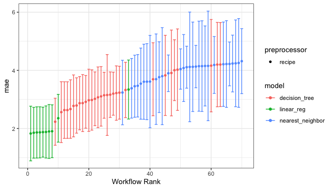
or the best from each workflow:
autoplot(chi_models, select_best = TRUE)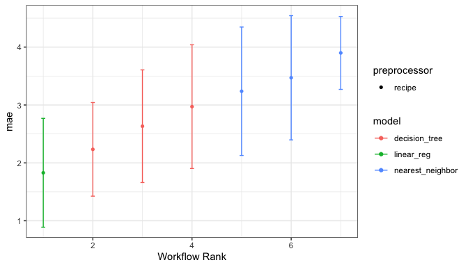
We can determine how well each combination did by looking at the best results per workflow:
rank_results(chi_models, rank_metric = "mae", select_best = TRUE) |>
  select(rank, mean, model, wflow_id, .config)
#> # A tibble: 7 × 5
#>    rank  mean model            wflow_id      .config
#>   <int> <dbl> <chr>            <chr>         <chr>
#> 1     1  1.83 linear_reg       simple_glmnet Preprocessor1_Model10
#> 2     2  2.23 decision_tree    simple_cart   Preprocessor1_Model06
#> 3     3  2.63 decision_tree    filter_cart   Preprocessor06_Model1
#> 4     4  2.97 decision_tree    pca_cart      Preprocessor4_Model2
#> 5     5  3.24 nearest_neighbor simple_knn    Preprocessor1_Model02
#> 6     6  3.47 nearest_neighbor filter_knn    Preprocessor06_Model1
#> 7 7 3.90 nearest_neighbor pca_knn Preprocessor2_Model2This project is released with a Contributor Code of Conduct. By contributing to this project, you agree to abide by its terms.
For questions and discussions about tidymodels packages, modeling, and machine learning, please post on Posit Community.
If you think you have encountered a bug, please submit an issue.
Either way, learn how to create and share a reprex (a minimal, reproducible example), to clearly communicate about your code.
Check out further details on contributing guidelines for tidymodels packages and how to get help.