README

twig is an R package for building decision and cost-effectiveness analyses. Below we provide instructions to install the twig R package, a simple Markov model example, and reference two cost-effectivenss tutorials, one on a time-dependent Markov model and the other on a decision tree. For building twig syntax interactively, you can use DecisionTwig which is an online graphical user interface for developing twig syntax.

Installation

A CRAN version will soon be available. Meanwhile, to install twig from GitHub, use the following command in R:

library(devtools)
install_github("hjalal/twig")

Overview

twig streamlines the process of building models by defining a Grammar of Modeling inspired by the Grammar of Graphics used in the ggplot2 package. twig leverages vectorized operations for efficiency.

A minimal example:

library(twig)
mytwig <- twig() + 
  decisions(names = c("A", "B")) +  # Decision alternatives
  states(names = c("Alive", "Dead"),  # Markov state names
         init_probs = c(1, 0)) +  # The cohort starts healthy
  event(name = "death_event",  # A death event can   
        options = c("yes", "none"),  # have two options: "yes" and "none",
        probs = c(pDie, leftover),  # occur with probabilities: pDie and leftover = 1 - pDie
        transitions=c(Dead,stay)) + # can lead to death state otherwise stay in their current state, respectively.
  payoffs(names = c(cost, utility))  # Payoff function names

The concept of Grammar of Modeling is insipred by ggplot’s Grammar of Graphics. The key benefit of adopting this grammar is to minimize repetition in decision and cost-effectiveness analysis modeling to streamline model building, maintenance and debugging. The twig above consists of a decisions layer that includes the names of the alternative strategies or choices, a states layer that describes the Markov states and their initial probabilities, an event layer die_event, and finally a payoffs layer describing how payoffs are accumulated.

The key component of the Grammar of Modeling is to develop a generic sequence of events a twig that applies to the entire population. The flow through these events can be controlled by the probability functions probs which can depend on the decision, state, cycle, cycle_in_state for tunnels and prior events in the twig

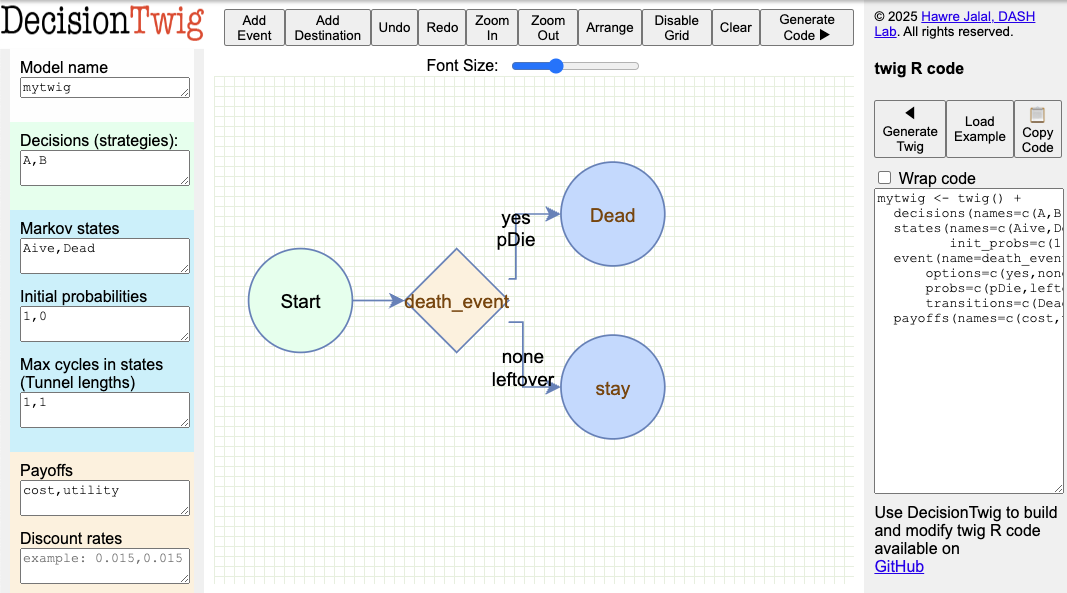
DecisionTwig

DecisionTwig allows to interactively build the twig syntax. This can be especially helpful for more complex event sequence structure.

Vectorized functions

Next, we define the three functions that we used in the twig: pDie, cost and utility. Note that these functions are all vectorized, meaning that they can take a vector of states, decisions, and parameters and return a vector of probabilities, costs, and utilities. This is a key feature of twig that allows for efficient computation of the model across multiple simulations.

# 1. probability of death is a function of the state, decision and relative risk of mortality given treatment A
pDie <- function(state, decision, rrMortA){
  rDie <- 0.01*(state=="Alive") * rrMortA^(decision=="A") # rate of death is 20% if alive, 0 otherwise. This rate is multiplied by rrMortA for A, otherwise 1.
  rate2prob(rDie) # convert the rate into probability
}

# 2. cost is a function of the decision
cost <- function(decision, cA, cB){
  cA * (decision=="A") + 
  cB * (decision=="B")
}

# 3. utility is uAlive if alive, otherwise 0
utility <- function(state, uAlive){
  uAlive * (state=="Alive")
}

Here we use a concise way to define if statements. For example, cA * (decision=="A") is equivalent to ifelse(decision=="A", cA, 0). Both statements are vectorized and can take a vector of decisions and return a vector of costs. However, the former is more concise and easier to read because it avoids nesting multiple ifelse statements.

We also used rrMortA^(decision=="A") to apply the relative risk of mortality if the decision is A, otherwise 1. This is because decision=="A" is treated as 1, and decision!="A" is treated as 0. By combining * and ^ we can concisely express multiple conditional statements.

Parameters

Then, we can define our parameters as a probabilistic dataset of the parameters:

n_sims <- 1000 # number of simulations

psa_params <- data.frame(
  rrMortA = rnorm(n_sims, 0.9, 0.1), # Normal: relative risk of mortality
  cA = rlnorm(n_sims, 6, 1), # Log-normal: cost of A
  cB = rlnorm(n_sims, 5, 1), # Log-normal: cost of B
  uAlive = rbeta(n_sims, 0.8, 0.2)) # Beta: utility of being alive

head(psa_params) # examining the first 6 samples

#     rrMortA         cA        cB    uAlive
# 1 1.0168738 1270.91187  34.93591 0.9999919
# 2 0.8952317 1433.50158 351.25445 0.9497743
# 3 0.7524302   90.52039 273.80137 0.9999980
# 4 0.8276866  245.09993 488.33008 0.9805013
# 5 0.8751724   52.21374 219.23235 0.8402547
# 6 0.9473632  396.90634 112.18042 0.9991721

Lastly, we run the model for 50 cycles (years) and compute the average expected values (EV) for the costs and utilities of both strategies.

results <- run_twig(twig_obj = mytwig, params = psa_params, n_cycles = 50)

results$mean_ev #average across all simulations
#         payoff
# decision     cost  utility
#        A 32379.32 32.11033
#        B 12503.32 31.32062

Note that your results may be slightly different due to the randomness params.

Incremental Cost-Effectiveness Ratio (ICER):

We can produce the incremental cost-effectiveness ratio (ICER) by adapting dampack’s calculate_icer function:

# calculate_icers(results$mean_ev)
#   decision     cost  utility inc_cost inc_utility     ICER status
# B        B 12503.32 31.32062       NA          NA       NA     ND
# A        A 32379.32 32.11033 19875.99   0.7897148 25168.57     ND

Cost-Effectiveness Acceptability Curve (CEAC):

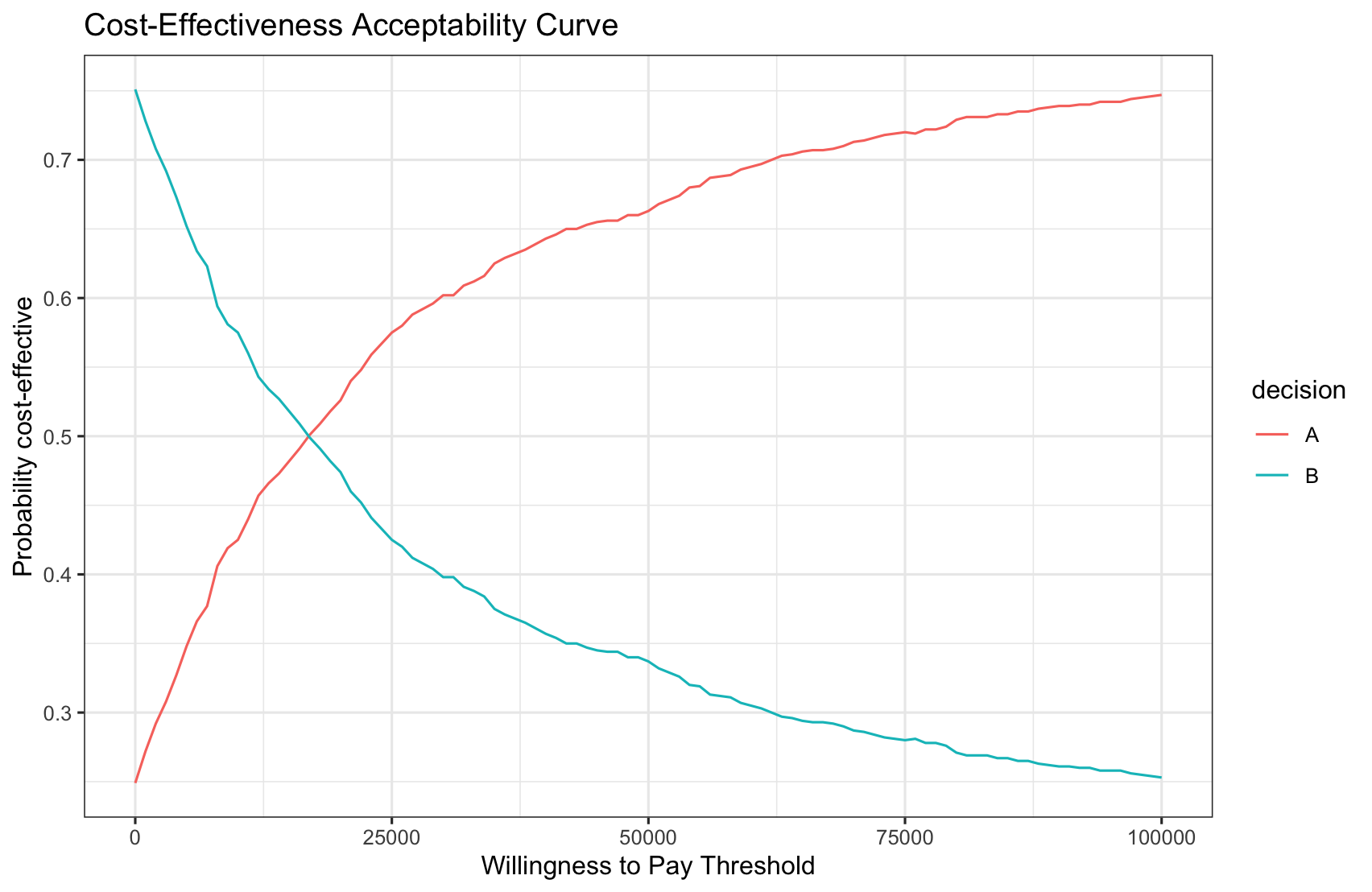
We can also plot the cost-effectiveness acceptability curve (CEAC) using a range of willingness to pay (WTP) thresholds:

plot_ceac(results$sim_ev, wtp_range = seq(0, 100000, by = 1000))

This brief tutorial demonstrated the basic functionality of the twig package with a simple Markov model. It shows how to define a simple twig, define the probabilistic input data, run the model, create the ICER table, and produce the CEAC curves. To illustrate more advanced functionality of twig, we provide two vignettes:

Additional Resources:

Disclaimer

Please note that both DecisionTwig and twig are still under active development and are provided as-is without any warranty.

`twig`

Getting started