![]()
![]()
![]()
tidyvpc provides a flexible and comprehensive toolkit
for parameterizing a Visual Predictive Check (VPC) in R. With
tidyverse style syntax, you can chain together functions
(e.g., %>% or |>) to easily perform
stratification, censoring, prediction correction, and more.
tidyvpc supports both continuous and categorical VPC.
# CRAN
install.packages("tidyvpc")

# Development
# If there are errors (converted from warning) during installation related to packages
# built under different version of R, they can be ignored by setting the environment variable
# R_REMOTES_NO_ERRORS_FROM_WARNINGS="true" before calling remotes::install_github()

Sys.setenv(R_REMOTES_NO_ERRORS_FROM_WARNINGS="true")
remotes::install_github("certara/tidyvpc")tidyvpcThe Certara.VPCResults
package offers a Shiny app that can be used to easily generate the
underlying tidyvpc and ggplot2 code used to
create your VPC.
After importing the observed and simulated data into your R
environment, use the function vpcResultsUI()
to parameterize the VPC and customize the resulting plot output using
the Shiny GUI - then generate the R code to reproduce from command
line!
install.packages("Certara.VPCResults",
                 repos = c("https://certara.jfrog.io/artifactory/certara-cran-release-public/",
                           "https://cloud.r-project.org"),
                 method = "libcurl")

library(tidyvpc)
library(Certara.VPCResults)

vpcResultsUI(observed = obs_data[MDV == 0], simulated = sim_data[MDV == 0])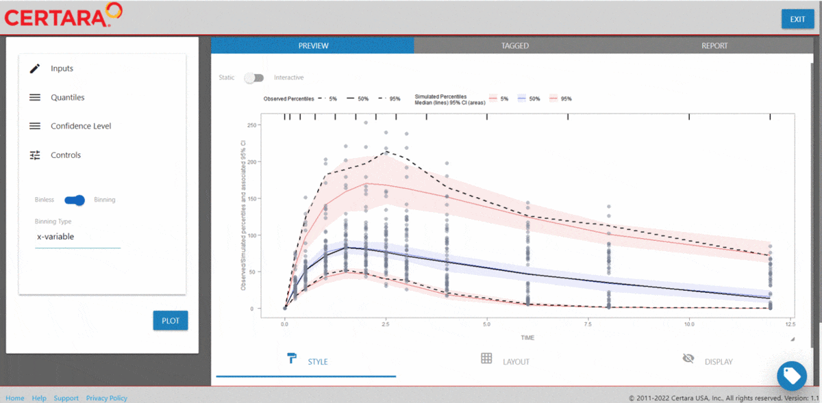
The Shiny application can serve as a learning heuristic and ensures
reproducibility by allowing you to save R and/or
Rmd scripts. Additionally, you may render RMarkdown to an
html, pdf, or docx output report.
Click here to
learn more about Certara.VPCResults.
tidyvpc requires a specific structure of observed and
simulated data in order to successfully generate VPC.
MDV == 0See tidyvpc::obs_data and tidyvpc::sim_data
for example data structures.
library(magrittr)
library(ggplot2)
library(tidyvpc)

# Filter MDV = 0
obs_data <- tidyvpc::obs_data[MDV == 0]
sim_data <- tidyvpc::sim_data[MDV == 0]

#Add LLOQ for each Study
obs_data$LLOQ <- obs_data[, ifelse(STUDY == "Study A", 50, 25)]

# Binning Method on x-variable (NTIME)
vpc <- observed(obs_data, x=TIME, y=DV) %>%
    simulated(sim_data, y=DV) %>%
    censoring(blq=(DV < LLOQ), lloq=LLOQ) %>%
    stratify(~ STUDY) %>%
    binning(bin = NTIME) %>%
    vpcstats()
Plot Code:
ggplot(vpc$stats, aes(x=xbin)) +
    facet_grid(~ STUDY) +
    geom_ribbon(aes(ymin=lo, ymax=hi, fill=qname, col=qname, group=qname), alpha=0.1, col=NA) +
    geom_line(aes(y=md, col=qname, group=qname)) +
    geom_line(aes(y=y, linetype=qname), size=1) +
    geom_hline(data=unique(obs_data[, .(STUDY, LLOQ)]),
        aes(yintercept=LLOQ), linetype="dotted", size=1) +
    geom_text(data=unique(obs_data[, .(STUDY, LLOQ)]),
        aes(x=10, y=LLOQ, label=paste("LLOQ", LLOQ, sep="="),), vjust=-1) +
    scale_colour_manual(
        name="Simulated Percentiles\nMedian (lines) 95% CI (areas)",
        breaks=c("q0.05", "q0.5", "q0.95"),
        values=c("red", "blue", "red"),
        labels=c("5%", "50%", "95%")) +
    scale_fill_manual(
        name="Simulated Percentiles\nMedian (lines) 95% CI (areas)",
        breaks=c("q0.05", "q0.5", "q0.95"),
        values=c("red", "blue", "red"),
        labels=c("5%", "50%", "95%")) +
    scale_linetype_manual(
        name="Observed Percentiles\n(black lines)",
        breaks=c("q0.05", "q0.5", "q0.95"),
        values=c("dotted", "solid", "dashed"),
        labels=c("5%", "50%", "95%")) +
    guides(
        fill=guide_legend(order=2),
        colour=guide_legend(order=2),
        linetype=guide_legend(order=1)) +
    theme(
        legend.position="top",
        legend.key.width=grid::unit(1, "cm")) +
    labs(x="Time (h)", y="Concentration (ng/mL)")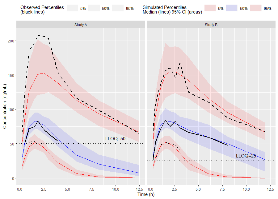
Or use the built-in plot() function from the
tidyvpc package.
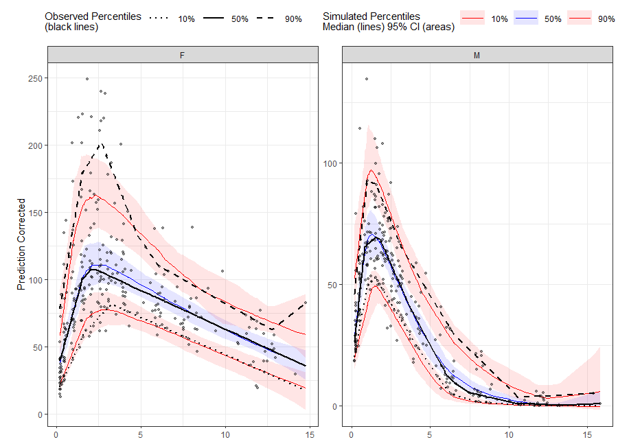
# Binless method using 10%, 50%, 90% quantiles and LOESS Prediction Corrected

# Add PRED variable to observed data from first replicate of sim_data
obs_data$PRED <- sim_data[REP == 1, PRED]

vpc <- observed(obs_data, x=TIME, y=DV) %>%
    simulated(sim_data, y=DV) %>%
    stratify(~ GENDER) %>%
    predcorrect(pred=PRED) %>%
    binless(loess.ypc = TRUE) %>%
    vpcstats(qpred = c(0.1, 0.5, 0.9))

plot(vpc)