The staggered R package computes the efficient estimator for settings with randomized treatment timing, based on the theoretical results in Roth and Sant’Anna (2023). If units are randomly (or quasi-randomly) assigned to begin treatment at different dates, the efficient estimator can potentially offer substantial gains over methods that only impose parallel trends. The package also allows for calculating the generalized difference-in-differences estimators of Callaway and Sant’Anna (2021) and Sun and Abraham (2021) and the simple-difference-in-means as special cases. There is a Stata implementation here. (We also previously wrote a Stata implementation via the RCall package, but recommend the native Stata package in the previous link.)
You can install the package from GitHub with:
# install.packages("devtools")
devtools::install_github("jonathandroth/staggered")We now illustrate how to use the package by re-creating some of the results in the application section of Roth and Sant’Anna (2021). Our data contains a balanced panel of police officers in Chicago who were randomly given a procedural justice training on different dates.
We first load the staggered package as well as some auxiliary packages for modifying and plotting the results.
library(staggered) #load the staggered package
library(ggplot2)   #load ggplot2 for plotting the results
#> Warning: package 'ggplot2' was built under R version 4.3.1

df <- staggered::pj_officer_level_balanced #load the officer dataWe now can call the function
calculate_adjusted_estimator_and_se to calculate the
efficient estimator. With staggered treatment timing, there are several
ways to aggregate treatment effects across cohorts and time periods. The
following block of code calculates the simple, calendar-weighted, and
cohort-weighted average treatment effects (see Section 2.3 of Roth and Sant’Anna (2021)
for more about different aggregation schemes).
#Calculate efficient estimator for the simple weighted average
staggered(df = df,
          i = "uid",
          t = "period",
          g = "first_trained",
          y = "complaints",
          estimand = "simple")
#>       estimate          se   se_neyman
#> 1 -0.001126981 0.002115194 0.002119248
#Calculate efficient estimator for the cohort weighted average
staggered(df = df,
i = "uid",
t = "period",
g = "first_trained",
y = "complaints",
estimand = "cohort")
#> estimate se se_neyman
#> 1 -0.001084689 0.002261011 0.002264876#Calculate efficient estimator for the calendar weighted average
staggered(df = df,
i = "uid",
t = "period",
g = "first_trained",
y = "complaints",
estimand = "calendar")
#> estimate se se_neyman
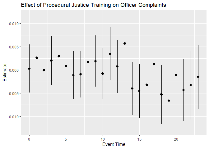
#> 1 -0.00187198 0.00255863 0.002561472We can also calculate an “event-study” that computes the average-treatment effect at each lag since treatment.
#Calculate event-study coefficients for the first 24 months (month 0 is instantaneous effect)
eventPlotResults <- staggered(df = df,
                              i = "uid",
                              t = "period",
                              g = "first_trained",
                              y = "complaints",
                              estimand = "eventstudy",
                              eventTime = 0:23)

head(eventPlotResults)
#>        estimate          se   se_neyman eventTime
#> 1  3.083575e-04 0.002645327 0.002650957         0
#> 2  2.591678e-03 0.002614563 0.002621513         1
#> 3 -4.872562e-05 0.002622640 0.002623634         2
#> 4  2.043434e-03 0.002715695 0.002720467         3
#> 5  2.977076e-03 0.002653917 0.002659630         4
#> 6  7.979656e-04 0.002721784 0.002727140         5
#Create event-study plot from the results of the event-study
eventPlotResults$ymin_ptwise <- with(eventPlotResults, estimate + 1.96 * se)
eventPlotResults$ymax_ptwise <- with(eventPlotResults, estimate - 1.96 * se)
ggplot(eventPlotResults, aes(x=eventTime, y =estimate)) +
geom_pointrange(aes(ymin = ymin_ptwise, ymax = ymax_ptwise))+
geom_hline(yintercept =0) +
xlab("Event Time") + ylab("Estimate") +
ggtitle("Effect of Procedural Justice Training on Officer Complaints")
The staggered package also allows you to calculate p-values using permutation tests, also known as Fisher Randomization Tests. These tests are based on a studentized statistic, and thus are finite-sample exact for the null of no treatment effects and asymptotically correct for the null of no average treatment effects.
#Calculate efficient estimator for the simple weighted average
#Use Fisher permutation test with 500 permutation draws
staggered(df = df,
          i = "uid",
          t = "period",
          g = "first_trained",
          y = "complaints",
          estimand = "simple",
          compute_fisher = T,
          num_fisher_permutations = 500)
#>       estimate          se   se_neyman fisher_pval fisher_pval_se_neyman
#> 1 -0.001126981 0.002115194 0.002119248       0.642                 0.644
#>   num_fisher_permutations
#> 1 500Our package also allows for the calculation of several other estimators proposed in the literature. For convenience we provide special functions for implementing the estimators proposed by Callaway & Sant’Anna and Sun & Abraham. The syntax is nearly identical to that for the efficient estimator:
#Calculate Callaway and Sant'Anna estimator for the simple weighted average
staggered_cs(df = df,
             i = "uid",
             t = "period",
             g = "first_trained",
             y = "complaints",
             estimand = "simple")
#>       estimate          se   se_neyman
#> 1 -0.005176818 0.003928735 0.003930919
#Calculate Sun and Abraham estimator for the simple weighted average
staggered_sa(df = df,
i = "uid",
t = "period",
g = "first_trained",
y = "complaints",
estimand = "simple")
#> estimate se se_neyman
#> 1 0.01153851 0.01730161 0.01730234The Callaway and Sant’Anna estimator corresponds with calling the
staggered function with beta=1 (and the default
use_DiD_A0=1), and the Sun and Abraham estimator
corresponds with calling staggered with beta=1 and
use_last_treated_only=T. If one is interested in the simple
difference-in-means, one can call the staggered function with option
beta=0.
Note that the standard errors returned in the se column are based on
the design-based approach in Roth & Sant’Anna, and thus will differ
somewhat from those returned by the did package. The
standard errors in se_neyman should be very similar to
those returned by the did package, although not identical in finite
samples.
We also provide a Stata implementation (staggered_stata)
via the RCall package, which calls the staggered R package from within
Stata. As mentioned above, we now have a native Stata
implementation which we recommend using over
staggered_stata. However, the instructions are
preserved below for backwards compatibility.
To install the staggered_stata package, the user first
needs to install the github and RCall packages. This can be done with
the following commands
> net install github, from("https://haghish.github.io/github/")
> github install haghish/rcall, version("2.5.0")
Important note: the staggered_stata
package was built under Rcall version 2.5.0, and the recent release of
RCall version 3.0 has created some compatibility issues. We will try our
best to fix these issues, but in the meantime it is best to install
version 2.5.0, as in the command above.
Note that the user must have R installed before installing the RCall
package. The latest version of R can be downloaded here. The
staggered_stata package can then be installed with
> github install jonathandroth/staggered_stataThe three packages can also be installed by downloading the ado files from the package webpages (github, RCall, staggered_stata) directly and pasting them into the user’s ado/personal directory.
The syntax for staggered_stata is very similar to that
for the staggered R package. Below are a few illustrative examples,
using the same data as above.
>use "https://github.com/jonathandroth/staggered_stata/raw/master/pj_officer_level_balanced.dta"
>staggered, y("complaints") g("first_trained") t("period") i("uid") estimand("simple")
>staggered_cs, y("complaints") g("first_trained") t("period") i("uid") estimand("eventstudy") eventTimeStart(-2) eventTimeEnd(2)
>staggered_sa, y("complaints") g("first_trained") t("period") i("uid") estimand("cohort")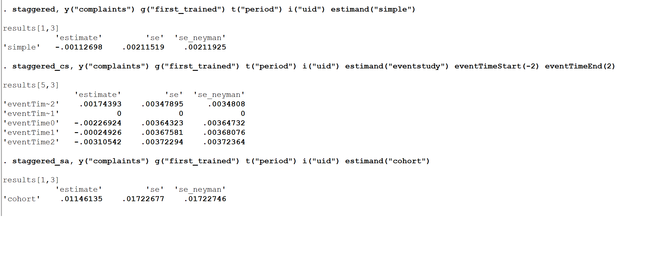
The staggered, staggered_cs, and
staggered_as commands all return a vector of coefficients
and covariance matrix in ereturn list, and thus can be used with any
post-estimation command in Stata (e.g. coefplot).