#> Warning: package 'ggplot2' was built under R version 4.1.2![]()

The R package splithalf provides tools
to estimate the internal consistency reliability of cognitive measures.
In particular, the tools were developed for application to tasks that
use difference scores as the main outcome measure, for instance the
Stroop score or dot-probe attention bias index (average RT in
incongruent trials minus average RT in congruent trials).
The methods in splithalf are built around split half reliability estimation. To increase the robustness of these estimates, the package implements a permutation approach that takes a large number of random (without replacement) split halves of the data. For each permutation the correlation between halves is calculated, with the Spearman-Brown correction applied (Spearman 1904). This process generates a distribution of reliability estimates from which we can extract summary statistics (e.g. average and 95% HDI).
While many cognitive tasks yield robust effects (e.g. everybody shows a Stroop effect) they may not yield reliable individual differences (Hedge, Powell, and Sumner 2018). As these measures are used in questions of individual differences researchers need to have some psychometric information for the outcome measures. Recently, it was proposed that psychological science should set a standard expectation for the reporting of reliability information for cognitive and behavioural measures (Parsons, Kruijt, and Fox 2019). splithalf was developed to support this proposition by providing a tool to easily extract internal consistency reliability estimates from behavioural measures.
The latest release version (0.7.2 unofficial version
name: Kitten Mittens) can be installed from CRAN:
install.packages("splithalf")The current developmental version (0.8.1 unofficial
version name: Rum Ham) can be installed from Github with:
devtools::install_github("sdparsons/splithalf")splithalf requires the tidyr
(Wickham and Henry 2019) and dplyr (Wickham et
al. 2018) packages for data handling within the functions. The
robustbase package is used to extract median scores
when applicable. The computationally heavy tasks (extracting many random
half samples of the data) are written in c++ via the
R package Rcpp (Eddelbuettel et al. 2018).
Figures use the ggplot package (Wickham 2016),
raincloud plots use code adapted from Allen et al. (Allen et al. 2019),
and the patchwork package (Pedersen 2019) is used for
plotting the multiverse analyses.
Citing packages is one way for developers to gain some recognition for the time spent maintaining the work. I would like to keep track of how the package is used so that I can solicit feedback and improve the package more generally. This would also help me track the uptake of reporting measurement reliability over time.
Please use the following reference for the code: Parsons, S., (2021). splithalf: robust estimates of split half reliability. Journal of Open Source Software, 6(60), 3041, https://doi.org/10.21105/joss.03041
Developing the splithalf package is a labour of love (and occasionally burning hatred). If you have any suggestions for improvement, additional functionality, or anything else, please contact me (sam.parsons@psy.ox.ac.uk) or raise an issue on github (https://github.com/sdparsons/splithalf). Likewise, if you are having trouble using the package (e.g. scream fits at your computer screen – we’ve all been there) do contact me and I will do my best to help as quickly as possible. These kind of help requests are super welcome. In fact, the package has seen several increases in performance and usability due to people asking for help.
Version 0.8.1 now out! [unofficial version name: “Rum Ham”] Lots of fixed issues in the multiverse functions, and lots more documentation/examples!
Now on github and submitted to CRAN: VERSION 0.7.2 [unofficial version name: “Kitten Mittens”] Featuring reliability multiverse analyses!!!
This update includes the addition of reliability multiverse functions. A splithalf object can be inputted into splithalf.multiverse to estimate reliability across a user-defined list of data-processing specifications (e.g. min/max RTs). Then, because sometimes science is more art than science, the multiverse output can be plotted with multiverse.plot. A brief tutorial can be found below, and a more comprehensive one can be found in a recent preprint (Parsons 2020).
Additionally, the output of splithalf has been reworked. Now a list is returned including the specific function calls, the processed data.
Since version 0.6.2 a user can also set plot = TRUE in
splithalf to generate a raincloud plot of the distribution of
reliability estimates.
It is important that we have a similar understanding of the terminology I use in the package and documentation. Each is also discussed in reference to the functions later in the documentation.
The core function splithalf requires that the input dataset has already undergone preprocessing (e.g. removal of error trials, RT trimming, and participants with high error rates). Splithalf should therefore be used with the same data that will be used to calculate summary scores and outcome indices. The exception is in multiverse analyses, as described below.
For those unfamiliar with R, the following snippets may help with common data-processing steps. I also highly recommend the Software Carpentry course “R for Reproducible Scientific Analysis” (https://swcarpentry.github.io/r-novice-gapminder/).
Note == indicates ‘is equal to,’ :: indicates that the function uses the package indicated, in the first case the dplyr package (Wickham et al. 2018).
dataset %>%
  dplyr::filter(accuracy == 1) %>%       ## keeps only trials in which participants made an accurate response
  dplyr::filter(RT >= 100, RT <= 2000)  %>%   ## removes RTs less than 100ms and greater than 2000ms
  dplyr::filter(participant != c(“p23”, “p45”)    ## removes participants “p23” and “p45”
If following rt trims you also trimmed by SD, use the following as well. Note that this is for two standard deviations from the mean, within each participant, and within each condition and trialtype.
dataset %>%
    dplyr::group_by(participant, condition, compare) %>%
    dplyr::mutate(low =  mean(RT) - (2 * sd(RT)),
                  high = mean(RT) + (2 * sd(RT))) %>%
    dplyr::filter(RT >= low & RT <= high)
If you want to save yourself effort in running splithalf, you could also rename your variable (column) names to the function defaults using the following
dplyr::rename(dataset,
              RT = "latency",
              condition = FALSE,
              participant = "subject",
              correct = "correct",
              trialnum = "trialnum",
              compare = "congruency")
The following examples assume that you have already processed your data to remove outliers, apply any RT cutoffs, etc. A reminder: the data you input into splithalf should be the same as that used to create your final scores - otherwise the resultant estimates will not accurately reflect the reliability of your data.
These questions should feed into what settings are appropriate for your need, and are aimed to make the splithalf function easy to use.
Are you interested in response times, or accuracy rates?
Knowing this, you can set outcome = "RT", or
outcome = "accuracy"
Say that your response time based task has two trial types;
“incongruent” and “congruent.” When you analyse your data will you use
the average RT in each trial type, or will you create a difference score
(or bias) by e.g. subtracting the average RT in congruent trials from
the average RT in incongruent trials. The first can be called with
score = "average" and the second with
score = "difference".
A super common way is to split the data into odd and even trials.
Another is to split by the first half and second half of the trials.
Both approaches are implemented in the splithalf funciton.
However, I believe that the permutation splithalf approach is the most
applicable in general and so the default is
halftype = "random"
For this brief example, we will simulate some data for 60 participants, who each completed a task with two blocks (A and B) of 80 trials. Trials are also evenly distributed between “congruent” and “incongruent” trials. For each trial we have RT data, and are assuming that participants were accurate in all trials.
n_participants = 60 ## sample size
n_trials = 80
n_blocks = 2

sim_data <- data.frame(participant_number = rep(1:n_participants, each = n_blocks * n_trials),
                       trial_number = rep(1:n_trials, times = n_blocks * n_participants),
                       block_name = rep(c("A","B"), each = n_trials, length.out = n_participants * n_trials * n_blocks),
                       trial_type = rep(c("congruent","incongruent"), length.out = n_participants * n_trials * n_blocks),
                       RT = rnorm(n_participants * n_trials * n_blocks, 500, 200),
ACC = 1)This is by far the most common outcome measure I have come across, so lets start with that.
Our data will be analysed so that we have two ‘bias’ or ‘difference score’ outcomes. So, within each block, we will take the average RT in congruent trials and subtract the average RT in incongruent trials. Calculating the final scores for each participant and for each block separately could be done as follows:
library("dplyr")
library("tidyr")

sim_data %>%
  dplyr::group_by(participant_number, block_name, trial_type) %>%
  dplyr::summarise(average = mean(RT)) %>%
  tidyr::spread(trial_type, average) %>%
  dplyr::mutate(bias = congruent - incongruent)
# A tibble: 120 x 5
# Groups:   participant_number, block_name [120]
   participant_number block_name congruent incongruent   bias
                <int> <chr>          <dbl>       <dbl>  <dbl>
 1                  1 A               550.        430. 120.
 2                  1 B               512.        433.  78.9
 3                  2 A               525.        496.  28.6
 4                  2 B               488.        523. -35.2
 5                  3 A               457.        500. -43.6
 6                  3 B               478.        518. -39.3
 7                  4 A               492.        479.  13.1
 8                  4 B               593.        458. 135.
 9                  5 A               568.        565.   2.72
10                  5 B               485.        555. -70.3
# ... with 110 more rows
To estimate reliability with splithalf we run the following.
library("splithalf")

difference <- splithalf(data = sim_data,
                        outcome = "RT",
                        score = "difference",
                        conditionlist = c("A", "B"),
                        halftype = "random",
                        permutations = 5000,
                        var.RT = "RT",
                        var.condition = "block_name",
                        var.participant = "participant_number",
                        var.compare = "trial_type",
                        compare1 = "congruent",
                        compare2 = "incongruent",
                        average = "mean",
                        plot = TRUE)
condition n splithalf 95_low 95_high spearmanbrown SB_low SB_high
1 A 60 -0.06 -0.23 0.13 -0.10 -0.37 0.23
2 B 60 -0.13 -0.30 0.06 -0.22 -0.46 0.10Specifying plot = TRUE will also allow you to plot the
distributions of reliability estimates. you can extract the plot from a
saved object with e.g. difference$plot.
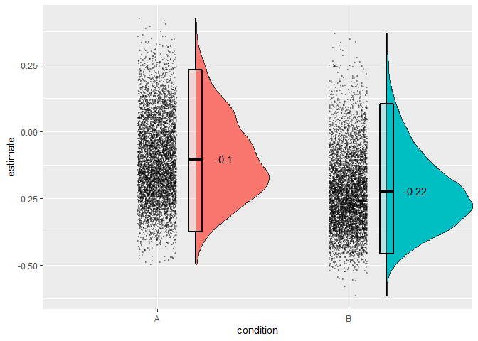
The splithalf output gives estimates separately for each condition defined (if no condition is defined, the function assumes that you have only a single condition, which it will call “all” to represent that all trials were included).
The second column (n) gives the number of participants analysed. If, for some reason one participant has too few trials to analyse, or did not complete one condition, this will be reflected here. I suggest you compare this n to your expected n to check that everything is running correctly. If the ns dont match, we have a problem. More likely, R will give an error message, but useful to know.
Next are the estimates; the splithalf column and the associated 95% percentile intervals, and the Spearman-Brown corrected estimate with its own percentile intervals. Unsurprisingly, our simlated random data does not yield internally consistant measurements.
What should I report? My preference is to report everything. 95% percentiles of the estimates are provided to give a picture of the spread of internal consistency estimates. Also included is the spearman-brown corrected estimates, which take into account that the estimates are drawn from half the trials that they could have been. Negative reliabilities are near uninterpretable and the spearman-brown formula is not useful in this case.
We estimated the internal consitency of bias A and B using a permutation-based splithalf approach (Parsons 2019) with 5000 random splits. The (Spearman-Brown corrected) splithalf internal consistency of bias A was were rSB = -0.1, 95%CI [-0.37,0.23].
— Parsons, 2020
For some tasks the outcome measure may simply be the average RT. In this case, we will ignore the trial type option. We will extract separate outcome scores for each block of trials, but this time it is simply the average RT in each block. Note that the main difference in this code is that we have omitted the inputs about what trial types to ‘compare,’ as this is irrelevant for the current task.
average <- splithalf(data = sim_data,
                     outcome = "RT",
                     score = "average",
                     conditionlist = c("A", "B"),
                     halftype = "random",
                     permutations = 5000,
                     var.RT = "RT",
                     var.condition = "block_name",
                     var.participant = "participant_number",
                     average = "mean")
condition n splithalf 95_low 95_high spearmanbrown SB_low SB_high
1 A 60 0.16 -0.02 0.34 0.26 -0.03 0.51
2 B 60 0.05 -0.13 0.24 0.09 -0.23 0.39The difference of differences score is a bit more complex, and perhaps also less common. I programmed this aspect of the package initially because I had seen a few papers that used a change in bias score in their analysis, and I wondered “I wonder how reliable that is as an individual difference measure.” Be warned, difference scores are nearly always less reliable than raw averages, and differences-of-differences will be less reliable again.
Our difference-of-difference variable in our task is the difference between bias observed in block A and B. So our outcome is calculated something like this.
BiasA = incongruent_A - congruent_A
BiasB = incongruent_B - congruent_B
Outcome = BiasB - BiasA
In our function, we specify this very similarly as in the difference score example. The only change will be changing the score to “difference_of_difference.” Note that we will keep the condition list consisting of A and B. But, specifying that we are interested in the difference of differences will lead the function to calculate the outcome scores apropriately.
diff_of_diff <- splithalf(data = sim_data,
                        outcome = "RT",
                        score = "difference_of_difference",
                        conditionlist = c("A", "B"),
                        halftype = "random",
                        permutations = 5000,
                        var.RT = "RT",
                        var.condition = "block_name",
                        var.participant = "participant_number",
                        var.compare = "trial_type",
                        compare1 = "congruent",
                        compare2 = "incongruent",
                        average = "mean")
condition n splithalf 95_low 95_high spearmanbrown
1 difference_of_difference score 60 -0.12 -0.29 0.07 -0.21
SB_low SB_high
1 -0.45 0.13This example is simplified from Parsons (2020). The process takes four steps. First, specify a list of data processing decisions. Here, we’ll specify only removing trials greater or lower than a specified amount. More options are available, such as total accuracy cutoff thresholds for participant removals.
specifications <- list(RT_min = c(0, 100, 200),
                       RT_max = c(1000, 2000),
                       averaging_method = c("mean", "median"))
Second, perform splithalf(...). The key difference here,
compared to the earlier examples is that we are no longer assuming that
all data processing has already occurred. Instead, the data processing
will be performed as part of splithalf.multiverse,
next.
difference <- splithalf(data = sim_data,
                        outcome = "RT",
                        score = "difference",
                        conditionlist = c("A"),
                        halftype = "random",
                        permutations = 5000,
                        var.RT = "RT",
                        var.condition = "block_name",
                        var.participant = "participant_number",
                        var.compare = "trial_type",
                        var.ACC = "ACC",
                        compare1 = "congruent",
                        compare2 = "incongruent",
                        average = "mean")
Third, perform splithalf.multiverse with the
specification list and splithalf objects as inputs
multiverse <- splithalf.multiverse(input = difference,
                                   specifications = specifications)
Finally, plot the multiverse with plot.multiverse.
multiverse.plot(multiverse = multiverse,
                title = "README multiverse")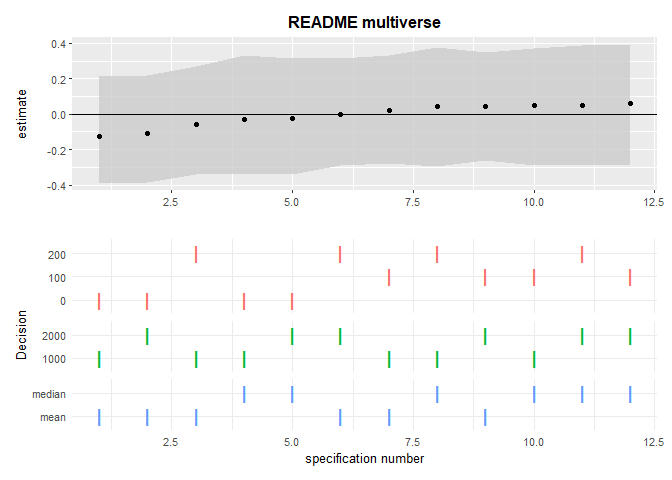
For more information, see Parsons (2020).
To examine how many random splits are required to provide a precise estimate, a short simulation was performed including 20 estimates of the spearman-brown reliability estimate, for each of 1, 10, 50, 100, 1000, 2000, 5000, 10000, and 20000 random splits. This simulation was performed on data from one block of 80 trials. Based on this simulation, I recommend 5000 (or more) random splits be used to calculate split-half reliability. 5000 permutations yielded a standard deviation of .002 and a total range of .008, indicating that the reliability estimates are stable to two decimal places with this number of random splits. Increasing the number of splits improved precision, however 20000 splits were required to reduce the standard deviation to .001.
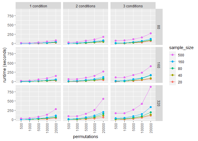
The speed of splithalf rests entirely on the number of
conditions, participants, and permutations. The biggest factor will be
your machine speed. For relative times, I ran a simulation with a range
of sample sizes, numbers of conditions, numbers of trials, and
permutations. The data is contained within the package as
data/speedtest.rda
The splithalf package is still under development. If you have suggestions for improvements to the package, or bugs to report, please raise an issue on github (https://github.com/sdparsons/splithalf). Currently, I have the following on my immediate to do list:
splithalf is the only package to implement all of
these tools, in particular reliability multiverse analyses. Some other
R packages offer a bootstrapped approach to split-half
reliability multicon (Sherman 2015),
psych (Revelle 2019), and splithalfr
(Pronk 2020)