![]()
![]()
![]()
![]()
You can install the latest CRAN version of soiltestcorr
with:
install.packages("soiltestcorr")Alternatively, you can install the development version of soiltestcorr from GitHub with:
# install.packages("devtools")
devtools::install_github("adriancorrendo/soiltestcorr")2.
Modified Arcsine-Log Calibration Curve
The goal of soiltestcorr is to assist users on
reproducible analysis of relationships between crop relative yield (ry)
and soil test values (stv) following different approaches.
The current available methods of correlation analysis in
soiltestcorr are:
The first method available is the Modified Arcsine-log Calibration
Curve (mod_alcc()) originally described by Dyson and
Conyers (2013) and modified by Correndo et al. (2017). This function
produces the estimation of critical soil test values (CSTV) for a target
relative yield (ry) with confidence intervals at adjustable confidence
levels.
mod_alcc()
Instructions
Load your data frame with soil test value (stv) and relative
yield (ry) data.
Specify the following arguments into the function -mod_alcc()-:
(a). data (optional),
(b). stv (soil test value) and ry (relative
yield) columns or vectors,
(c). target of relative yield (e.g. 90%),
(d). desired confidence level (e.g. 0.95 for 1 -
alpha(0.05)). Used for the estimation of critical soil test value (CSTV)
lower and upper limits.
(e). plot TRUE (produces a ggplot as main output) or
FALSE -default- (no plot, only results as list or tibble),
(f). tidy TRUE -default- (produces a tibble with
results) or FALSE (store results as list),
Run and check results.
Check residuals plot (see Section 3.3
SMA Residuals), and warnings related to potential leverage points.
Adjust curve plots as desired.
Example of mod_alcc() output
#> Warning: One or more original RY values exceeded 100%. All RY values greater
#>           than 100% have been capped to 100%.
#> Warning: 2 STV points exceeded the CSTV for 100% of RY.
#>   Risk of leverage. You may consider a sensitivity analysis by removing extreme points,
#>   re-run the mod_alcc(), and check results.
#> Warning: 2 STV points exceeded two-times (2x)
#>   the CSTV for 90% of RY. Risk of leverage. You may consider a sensitivity analysis by
#>   removing extreme points, re-run the mod_alcc(), and check results.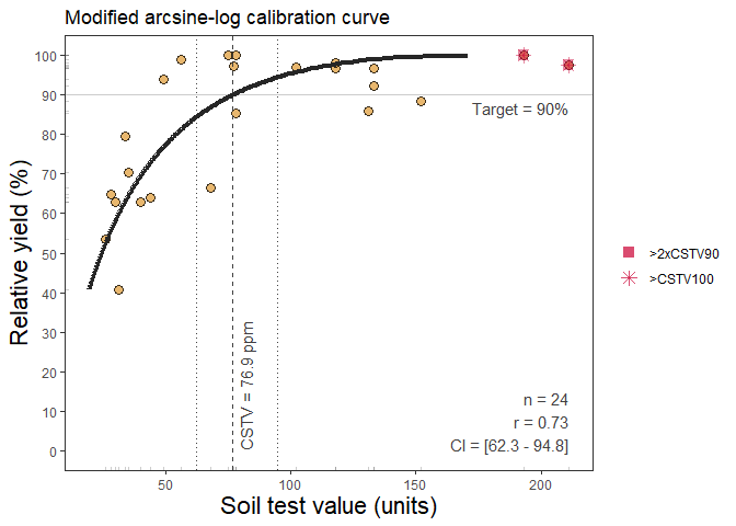
soiltestcorr also allows users to implement the
quadrants analysis approach, also known as the Cate-Nelson analysis.
There are two versions of the Cate-Nelson technique:
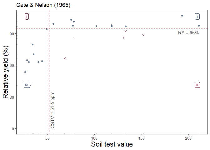
Thus, the second alternative is based on Cate and Nelson (1965)
(cate_nelson_1965()). The first step of this method is to
apply an arbitrarily fixed value of ry as a target (y-axis) that divides
the data into two categories (below & equal or above ry target). In
a second stage, it estimates the CSTV (x-axis) as the minimum stv that
divides the data into four quadrants (target ry level combined with STV
lower or greater than the CSTV) maximizing the number of points under
well-classified quadrants (II, stv >= CSTV & ry >= ry target;
and IV, stv < CSTV & ry < RY target). This is also known as
the “graphical” version of the Cate-Nelson approach.
cate_nelson_1965()
Instructions
Load your data frame with soil test value (stv) and relative
yield (ry) data.
Specify the following arguments into the function
-cate_nelson_1965()-:
(a). data (optional),
(b). stv (soil test value) and ry (relative
yield) columns or vectors,
(c). plot TRUE (produces a ggplot as main output) or
FALSE (no plot, only results as list or tibble),
(d). tidy TRUE-default- (produces a tibble with results)
or FALSE (store results as list),
Run and check results.
Adjust plot as desired.
Example of cate_nelson_1965() output
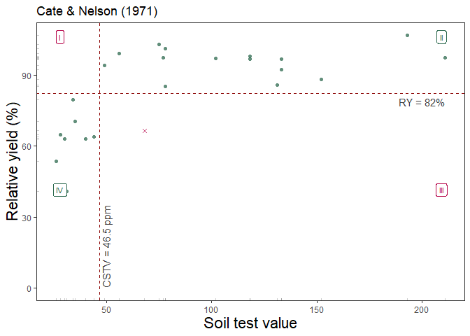
The third alternative is based on Cate and Nelson (1971)
(cate_nelson_1971()). The first step of this alternative
version is to estimate the CSTV (x-axis) as the minimum stv that
minimizes the residual sum of squares when dividing data points in two
classes (lower or greater than the CSTV) without using an arbitrary ry.
This refined version does not constrains the model performance (measured
with the coefficient of determination -R2-) but the user has no control
on the RY level for the CSTV. This is also known as the “statistical”
version of the Cate-Nelson approach.
cate_nelson_1971()
Instructions
Load your data frame with soil test value (stv) and relative
yield (ry) data.
Specify the following arguments into the function
-cate_nelson_1971()-:
(a). data (optional),
(b). stv (soil test value) and ry (relative
yield) columns or vectors,
(c). plot TRUE-default- (produces a ggplot as main
output) or FALSE (no plot, only results as list or tibble),
(d). tidy TRUE (produces a tibble with results) or FALSE
(store results as list),
Run and check results.
Adjust plot as desired.
Example of cate_nelson_1971() output
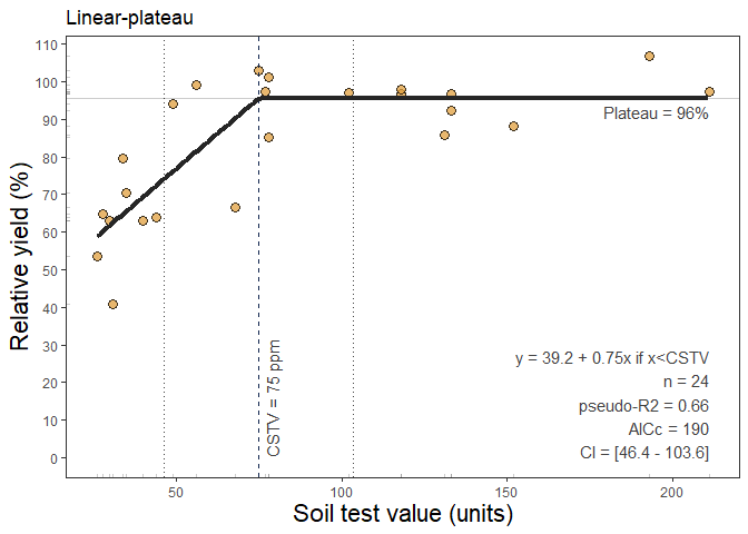
The next method available is the linear-plateau model
(linear_plateau()). This function fits the classical
regression response model that follows two phases: i) a first linear
phase described as y = a + b*x, and ii) a second
plateau-phase (Anderson and Nelson, 1975) were the ry
response to increasing stv becomes NULL (flat), described
as plateau = y = a + b*Xc, where y represents
the fitted crop relative yield, x the soil test value,
a the intercept (ry when stv = 0) , b the
slope (as the change in ry per unit of soil nutrient supply or nutrient
added), and X_c the join-point when the plateau-phase
starts (i.e. the CSTV). The linear_plateau() function works
automatically with self starting initial values to facilitate the
model’s convergence.
linear_plateau()
Instructions
Load your data frame or vectors with soil test value (stv) and
relative yield (ry) data.
Specify the following arguments into the function
-linear_plateau()-:
(a). data (optional),
(b). stv (soil test value) and ry (relative
yield) columns or vectors,
(c). target (optional) if want to know stv level needed
for a different `ry`` than the plateau.
(d). plot TRUE (produces a ggplot as main output) or
FALSE (no plot, only results as tibble),
(e). resid TRUE (produces plots with residuals analysis)
or FALSE (no plot),
(f). tidy TRUE-default- (produces a tibble with results)
or FALSE (store results as list),
Run and check results.
Check residuals plot, and warnings related to potential
limitations of this model.
Adjust curve plots as desired.
Example of linear_plateau() output
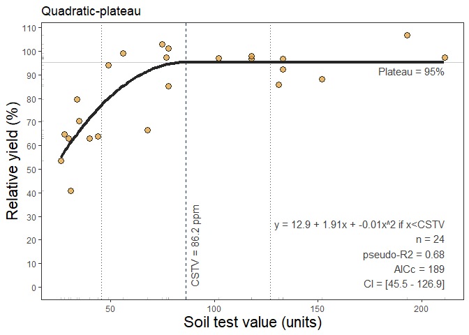
The following correlation method available is the quadratic-plateau
model (quadratic_plateau()). This function fits the
classical regression response model that follows two phases: i) a first
curvilinear phase described as y = a + b*x + c*x^2, and ii)
a second plateau-phase (Bullock and Bullock, 1994) were the
ry response to increasing stv becomes NULL
(flat), described as plateau = y = a + b*Xc + c*Xc, where
y represents the fitted crop relative yield, x
the soil test value, a the intercept (ry when stv = 0) ,
b the linear slope (as the change in ry per unit of soil
nutrient supply or nutrient added), c the quadratic
coefficient (giving the curve shape), and X_c the
join-point when the plateau-phase starts (i.e. the CSTV). The
quadratic_plateau() function works automatically with self
starting initial values to facilitate the model convergence.
quadratic_plateau()
Instructions
Load your data frame with soil test value (stv) and relative
yield (ry) data.
Specify the following arguments into the function
-quadratic_plateau()-:
(a). data (optional),
(b). stv (soil test value) and ry (relative
yield) columns or vectors,
(c). target (optional) if want to know stv level needed
for a different `ry`` than the plateau.
(d). plot TRUE (produces a ggplot as main output) or
FALSE (no plot, only results as tibble),
(e). resid TRUE (produces plots with residuals analysis)
or FALSE (no plot),
(f). tidy TRUE-default- (produces a tibble with results)
or FALSE (store results as list),
Run and check results.
Check residuals plot, and warnings related to potential
limitations of this model.
Adjust curve plots as desired.
Example of quadratic_plateau() output
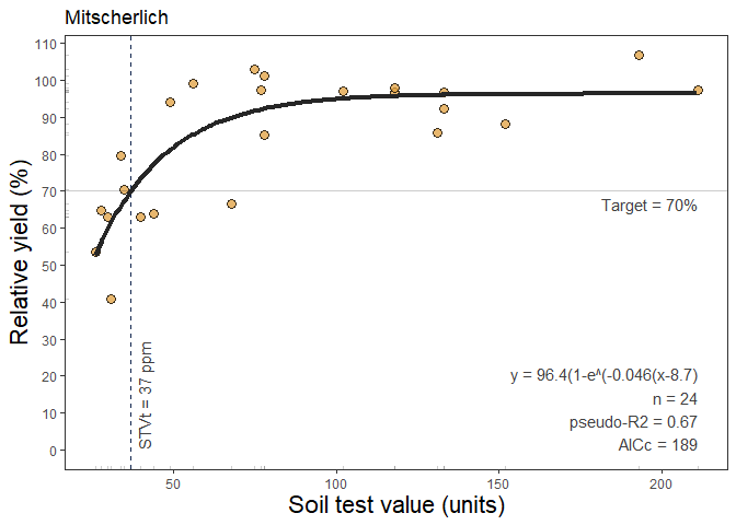
This function fits an exponential regression response model (Melsted
and Peck, 1977) that follows a curve shape described as
y = a * (1-exp(-c(x + b)), where
a = asymptote, b = xintercept,
c = rate or curvature parameter. The
mitscherlich() function works automatically with self
starting initial values to facilitate the model’s convergence. This
approach is extensively used in agriculture to describe crops response
to input since the biological meaning of its curved response. With 3
alternatives to fit the model, this function brings the advantage of
controlling the parameters quantity: i) type = 1 (DEFAULT),
corresponding to the model without any restrictions to the parameters
(y = a * (1-exp(-c(x + b))); ii) type = 2 (“asymptote
100”), corresponding to the model with only 2 parameters by setting the
asymptote = 100 (y = 100 * (1-exp(-c(x + b))), and iii)
type = 3 (“asymptote 100 from 0”), corresponding to the model with only
1 parameter by constraining the asymptote = 100 and xintercept = 0
(y = 100 * (1-exp(-c(x))).
Instructions
Load your data frame with soil test value (stv) and relative
yield (ry) data.
Specify the following arguments into the function
-mitscherlich()-:
(a). data (optional),
(b). stv (soil test value) and ry (relative
yield) columns or vectors,
(c). target (optional) if want to know stv level needed
for a specific ry.
(d). plot TRUE (produces a ggplot as main output) or
FALSE (no plot, only results as tibble),
(e). resid TRUE (produces plots with residuals analysis)
or FALSE (no plot),
(f). tidy TRUE-default- (produces a tibble with results)
or FALSE (store results as list),
Run and check results.
Check residuals plot, and warnings related to potential
limitations of this model.
Adjust curve plots as desired.
Example of mitscherlich() output
References
Anderson, R. L., and Nelson, L. A. (1975). A Family of Models
Involving Intersecting Straight Lines and Concomitant Experimental
Designs Useful in Evaluating Response to Fertilizer Nutrients.
Biometrics, 31(2), 303–318. 10.2307/2529422
Bullock, D.G. and Bullock, D.S. (1994), Quadratic and
Quadratic-Plus-Plateau Models for Predicting Optimal Nitrogen Rate of
Corn: A Comparison. Agron. J., 86: 191-195.
10.2134/agronj1994.00021962008600010033x
Cate, R.B. Jr., and Nelson, L.A., 1965. A rapid method for
correlation of soil test analysis with plant response data. North
Carolina Agric. Exp. Stn., International soil Testing Series Bull.
No. 1.
Cate, R.B. Jr., and Nelson, L.A., 1971. A simple statistical
procedure for partitioning soil test correlation data into two classes.
Soil Sci. Soc. Am. Proc. 35:658-659
Correndo, A.A., Salvagiotti, F., García, F.O. and Gutiérrez-Boem,
F.H., 2017. A modification of the arcsine–log calibration curve for
analysing soil test value–relative yield relationships. Crop and Pasture
Science, 68(3), pp.297-304. 10.1071/CP16444
Dyson, C.B., Conyers, M.K., 2013. Methodology for online
biometric analysis of soil test-crop response datasets. Crop &
Pasture Science 64: 435–441. 10.1071/CP13009
Melsted, S.W. and Peck, T.R. (1977). The Mitscherlich-Bray Growth
Function. In Soil Testing (eds T. Peck, J. Cope and D. Whitney).
10.2134/asaspecpub29.c1
Warton, D.I., Wright, I.J., Falster, D.S., and Westoby, M., 2006.
Bivariate line-fitting methods for allometry. Biol. Rev. Camb. Philos.
Soc. 81, 259–291. 10.1017/S1464793106007007