singleRcapture:
An R Package for Single-Source Capture-Recapture Models
singleRcapture:
An R Package for Single-Source Capture-Recapture Models
![]()
![]()
![]()
Capture-recapture type experiments are used to estimate the total population size in situations when observing only a part of such population is feasible. In recent years these types of experiments have seen more interest.
Single-source models are distinct from other capture-recapture models because we cannot estimate the population size based on how many units were observed in two or three sources which is the standard approach.
Instead in single-source models we utilize count data regression models on positive distributions (i.e. on counts greater than 0) where the dependent variable is the number of times a particular unit was observed in source data.
This package aims to implement already existing and introduce new methods of estimating population size from single source to simplify the research process.
Currently, we have implemented most of the frequentist approaches used in literature such as:
oichao() model
based on counts 2 and 3.ratioReg() support for ratio regression with
optional one-inflation model selection.For more details we see the
singleRcapture: An R Package for Single-Source Capture-Recapture Models
vignette on CRAN or pkgdown
website.
You can install the current version of the
singleRcapture package from main branch GitHub
with:
# install.packages("devtools")
remotes::install_github("ncn-foreigners/singleRcapture")
or install the stable version from CRAN with:
install.packages("singleRcapture")The main function of this package is estimatePopsize
which fits regression on specified distribution and then uses fitted
regression to estimate the population size.
Let’s look at a model from 2003 publication (Van Der Heijden, P. G.,
Bustami, R., Cruyff, M. J., Engbersen, G., & Van Houwelingen, H. C.
(2003). Point and interval estimation of the population size using the
truncated Poisson regression model. Statistical Modelling, 3(4),
305-322.). The call to estimatePopsize will look very
similar to anyone who used the stats::glm function:
library(singleRcapture)
model <- estimatePopsize(
  formula = capture ~ gender + age + nation, # specify formula
  data = netherlandsimmigrant,
  popVar = "analytic", # specify
  model = "ztpoisson", # distribution used
  method = "IRLS", # fitting method one of three currently supported
  controlMethod = controlMethod(silent = TRUE) # ignore convergence at half step warning
)
summary(model) # a summary method for singleR class with standard glm-like output and population size estimation results
#>
#> Call:
#> estimatePopsize.default(formula = capture ~ gender + age + nation,
#>     data = netherlandsimmigrant, model = "ztpoisson", method = "IRLS",
#>     popVar = "analytic", controlMethod = controlMethod(silent = TRUE))
#>
#> Pearson Residuals:
#>      Min.   1st Qu.    Median      Mean   3rd Qu.      Max.
#> -0.486442 -0.486442 -0.298080  0.002093 -0.209444 13.910844
#>
#> Coefficients:
#> -----------------------
#> For linear predictors associated with: lambda
#>                      Estimate Std. Error z value  P(>|z|)
#> (Intercept)           -1.3411     0.2149  -6.241 4.35e-10 ***
#> gendermale             0.3972     0.1630   2.436 0.014832 *
#> age>40yrs             -0.9746     0.4082  -2.387 0.016972 *
#> nationAsia            -1.0926     0.3016  -3.622 0.000292 ***
#> nationNorth Africa     0.1900     0.1940   0.979 0.327398
#> nationRest of Africa  -0.9106     0.3008  -3.027 0.002468 **
#> nationSurinam         -2.3364     1.0136  -2.305 0.021159 *
#> nationTurkey          -1.6754     0.6028  -2.779 0.005445 **
#> ---
#> Signif. codes:  0 '***' 0.001 '**' 0.01 '*' 0.05 '.' 0.1 ' ' 1
#>
#> AIC: 1712.901
#> BIC: 1757.213
#> Residual deviance: 1128.553
#>
#> Log-likelihood: -848.4504 on 1872 Degrees of freedom
#> Number of iterations: 8
#> -----------------------
#> Population size estimation results:
#> Point estimate 12690.35
#> Observed proportion: 14.8% (N obs = 1880)
#> Std. Error 2808.165
#> 95% CI for the population size:
#>           lowerBound upperBound
#> normal      7186.449   18194.25
#> logNormal   8431.277   19718.31
#> 95% CI for the share of observed population:
#>           lowerBound upperBound
#> normal     10.332933   26.16035
#> logNormal   9.534288   22.29793
We implemented a method for plot function to visualise
the model fit and other useful diagnostic information. One of which is
rootogram, a type of plot that compares fitted and observed
marginal frequencies:
plot(model, plotType = "rootogram")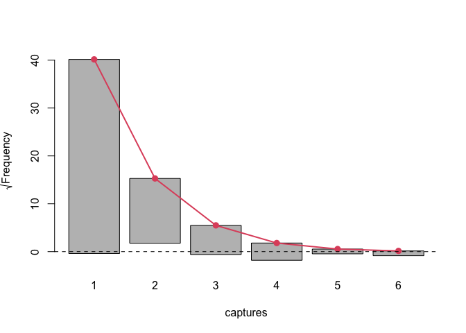
The possible values for plotType argument are:
qq - the normal quantile-quantile plot for pearson
residuals (default),marginal - a matplot comparing fitted and
observed marginal frequencies,fitresid - plot of linear predictor values contrasted
with pearson residuals,bootHist - histogram of bootstrap sample,rootogram - rootogram, example presented above,dfpopContr - contrasting two deletion effects to
identify presence of influential observations,dfpopBox - boxplot of results from
dfpopsize function see its documentation,scaleLoc - scale-location plot,cooks - plot of cooks.values for
distributions for which it is defined,hatplot - plot of hatvalues,strata - plot of confidence intervals for selected such
populations.User can also pass arguments to specify additional information such
as plot title, subtitle etc. similar to calling plot on
some data. For more info check plot.singleR method
documentation.
The package also includes a standalone ratioReg()
function for the ratio-regression approach. It is separate from
singleRmodels() because it works on neighbouring
marginal-frequency ratios rather than on unit-level count
likelihoods:
toyRatio <- data.frame(
  observed = c(rep(1, 50), rep(2, 30), rep(3, 15), rep(4, 6), rep(5, 2))
)

ratioModel <- ratioReg(
  observed ~ 1,
  data = toyRatio,
  model = "auto",
  estimator = "SM",
  confint = "none"
)

summary(ratioModel)
#>
#> Call:
#> ratioReg(formula = observed ~ 1, data = toyRatio, model = "auto",
#>     estimator = "SM", confint = "none")
#>
#> Selected ratio regression model: M1
#> Selection criterion: AIC
#> Primary population estimator: SM
#> Observed population size: 103
#>
#> Model selection table:
#>    model available logLik     AIC    BIC selected
#> M0    M0      TRUE   7.85  -9.701 -11.54    FALSE
#> M1    M1      TRUE  20.14 -32.284 -34.74     TRUE
#>
#> Coefficients for M0 :
#> (Intercept)  log(k + 1)
#>     -0.1035     -0.5724
#>
#> Coefficients for M1 :
#>  (Intercept)   log(k + 1) oneInflation
#>       0.1714      -0.7865      -0.1371
#>
#> Population size estimates:
#>  estimator pointEstimate variance lowerBound upperBound
#>         HT      139.7316       NA         NA         NA
#>         SM      139.7308       NA         NA         NA
The default ratio-regression plot shows the observed log-ratios
together with the fitted M0 and M1 curves:
plot(ratioModel)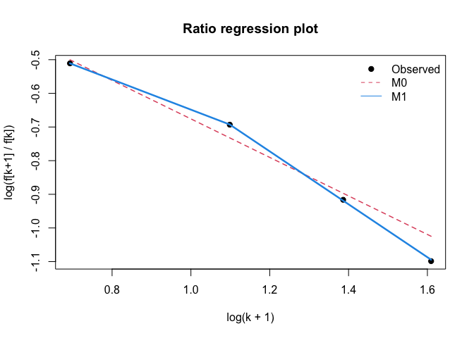
As we have seen there are some significant differences between fitted and observed marginal frequencies. To check our intuition let’s perform goodness of fit test between fitted and observed marginal frequencies.
To do it we call a summary function of
marginalFreq function which computes marginal frequencies
for the fitted singleR class object:
summary(marginalFreq(model), df = 2, dropl5 = "group")
#> Test for Goodness of fit of a regression model:
#>
#>                  Test statistics df P(>X^2)
#> Chi-squared test           50.06  2 1.3e-11
#> G-test                     34.31  2 3.6e-08
#>
#> --------------------------------------------------------------
#> Cells with fitted frequencies of < 5 have been grouped
#> Names of cells used in calculating test(s) statistic: 1 2 3
Finally let us check if we have any influential observations. We will do this by comparing the deletion effect of every observation on population size estimate by removing it entirely from the model (from population size estimate and regression) and by only omitting it in pop size estimation (this is what is called the contribution of an observation). If observation is not influential these two actions should have the approximately the same effect:
plot(model, plotType = "dfpopContr")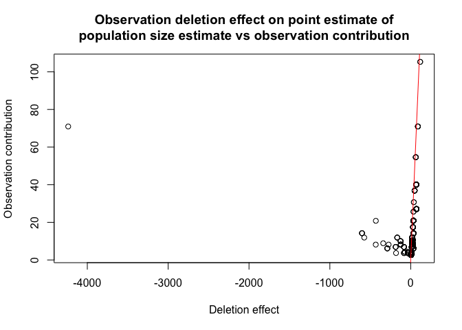
it is easy to deduce from the plot above that we have influential observations in our dataset (one in particular).
Lastly singleRcapture offers some post-hoc procedures
for example a function stratifyPopsize that estimates sizes
of user specified sub populations and returns them in a
data.frame:
stratifyPopsize(model, alpha = c(.01, .02, .03, .05), # different significance level for each sub population
    strata = list(
    "Females from Surinam" = netherlandsimmigrant$gender == "female" & netherlandsimmigrant$nation == "Surinam",
    "Males from Turkey" = netherlandsimmigrant$gender == "male" & netherlandsimmigrant$nation == "Turkey",
    "Younger males" = netherlandsimmigrant$gender == "male" & netherlandsimmigrant$age == "<40yrs",
    "Older males" = netherlandsimmigrant$gender == "male" & netherlandsimmigrant$age == ">40yrs"
))
#>                   name Observed Estimated ObservedPercentage  StdError
#> 1 Females from Surinam       20  931.4677           2.147149  955.0657
#> 2    Males from Turkey       78 1291.2513           6.040652  741.0066
#> 3        Younger males     1391 7337.0708          18.958520 1282.1402
#> 4          Older males       91 1542.1886           5.900705  781.4747
#>   normalLowerBound normalUpperBound logNormalLowerBound logNormalUpperBound
#> 1      -1528.61853         3391.554            119.2661            8389.158
#> 2       -432.58790         3015.090            405.4127            4573.791
#> 3       4554.71057        10119.431           5134.8122           10834.785
#> 4         10.52637         3073.851            630.7551            3992.674
#>   confLevel
#> 1      0.01
#> 2      0.02
#> 3      0.03
#> 4      0.05
strata argument may be specified in various ways for
example:
stratifyPopsize(model, strata = ~ gender / age)
#>                     name Observed Estimated ObservedPercentage  StdError
#> 1         gender==female      398 3811.0911          10.443203 1153.9733
#> 2           gender==male     1482 8879.2594          16.690581 1812.0790
#> 3 genderfemale:age<40yrs      378 3169.8263          11.924944  880.9478
#> 4   gendermale:age<40yrs     1391 7337.0708          18.958520 1282.1402
#> 5 genderfemale:age>40yrs       20  641.2648           3.118836  407.5264
#> 6   gendermale:age>40yrs       91 1542.1886           5.900705  781.4747
#>   normalLowerBound normalUpperBound logNormalLowerBound logNormalUpperBound
#> 1       1549.34513         6072.837           2189.0443            6902.133
#> 2       5327.64991        12430.869           6090.7762           13354.880
#> 3       1443.20030         4896.452           1904.3126            5484.617
#> 4       4824.12208         9850.019           5306.3306           10421.082
#> 5       -157.47223         1440.002            212.3382            2026.726
#> 6         10.52637         3073.851            630.7551            3992.674
#>   confLevel
#> 1      0.05
#> 2      0.05
#> 3      0.05
#> 4      0.05
#> 5      0.05
#> 6      0.05
The package was designed with convenience in mind, for example it is possible to specify that weights provided on call are to be interpreted as number of occurrences of units in each row:
df <- netherlandsimmigrant[, c(1:3,5)]
df$ww <- 0
### this is dplyr::count without dependencies
df <- aggregate(ww ~ ., df, FUN = length)
summary(estimatePopsize(
  formula = capture ~ nation + age + gender,
  data = df,
  model = ztpoisson,
  weights = df$ww,
  controlModel = controlModel(weightsAsCounts = TRUE)
))
#>
#> Call:
#> estimatePopsize.default(formula = capture ~ nation + age + gender,
#>     data = df, model = ztpoisson, weights = df$ww, controlModel = controlModel(weightsAsCounts = TRUE))
#>
#> Pearson Residuals:
#>      Min.   1st Qu.    Median      Mean   3rd Qu.      Max.
#> -317.6467   -2.4060    3.7702    0.0803   13.4920  183.2108
#>
#> Coefficients:
#> -----------------------
#> For linear predictors associated with: lambda
#>                      Estimate Std. Error z value  P(>|z|)
#> (Intercept)           -1.3411     0.2149  -6.241 4.35e-10 ***
#> nationAsia            -1.0926     0.3016  -3.622 0.000292 ***
#> nationNorth Africa     0.1900     0.1940   0.979 0.327398
#> nationRest of Africa  -0.9106     0.3008  -3.027 0.002468 **
#> nationSurinam         -2.3364     1.0136  -2.305 0.021159 *
#> nationTurkey          -1.6754     0.6028  -2.779 0.005445 **
#> age>40yrs             -0.9746     0.4082  -2.387 0.016972 *
#> gendermale             0.3972     0.1630   2.436 0.014832 *
#> ---
#> Signif. codes:  0 '***' 0.001 '**' 0.01 '*' 0.05 '.' 0.1 ' ' 1
#>
#> AIC: 1712.901
#> BIC: 1757.213
#> Residual deviance: 1128.553
#>
#> Log-likelihood: -848.4504 on 1872 Degrees of freedom
#> Number of iterations: 8
#> -----------------------
#> Population size estimation results:
#> Point estimate 12690.35
#> Observed proportion: 14.8% (N obs = 1880)
#> Std. Error 2808.169
#> 95% CI for the population size:
#>           lowerBound upperBound
#> normal      7186.444   18194.26
#> logNormal   8431.275   19718.32
#> 95% CI for the share of observed population:
#>           lowerBound upperBound
#> normal     10.332927   26.16037
#> logNormal   9.534281   22.29793
Methods such as regression diagnostics will be adjusted (values of weights will be reduced instead of rows being removed etc.)
We also included option to use common non standard argument such as significance levels different from usual 5%:
set.seed(123)
modelInflated <- estimatePopsize(
    formula = capture ~ gender + age,
    data = netherlandsimmigrant,
    model = "ztoigeom",
    method = "IRLS",
    # control parameters for population size estimation check documentation of controlPopVar
    controlPopVar = controlPopVar(
        alpha = .01, # significance level
    )
)
summary(modelInflated)
#>
#> Call:
#> estimatePopsize.default(formula = capture ~ gender + age, data = netherlandsimmigrant,
#>     model = "ztoigeom", method = "IRLS", controlPopVar = controlPopVar(alpha = 0.01,
#>         ))
#>
#> Pearson Residuals:
#>      Min.   1st Qu.    Median      Mean   3rd Qu.      Max.
#> -0.357193 -0.357193 -0.357193  0.000343 -0.287637 10.233608
#>
#> Coefficients:
#> -----------------------
#> For linear predictors associated with: lambda
#>             Estimate Std. Error z value P(>|z|)
#> (Intercept)  -1.5346     0.1846  -8.312 < 2e-16 ***
#> gendermale    0.3863     0.1380   2.800 0.00512 **
#> age>40yrs    -0.7788     0.2942  -2.648 0.00810 **
#> -----------------------
#> For linear predictors associated with: omega
#>             Estimate Std. Error z value  P(>|z|)
#> (Intercept)  -1.7591     0.3765  -4.673 2.97e-06 ***
#> ---
#> Signif. codes:  0 '***' 0.001 '**' 0.01 '*' 0.05 '.' 0.1 ' ' 1
#>
#> AIC: 1736.854
#> BIC: 1759.01
#> Residual deviance: 1011.271
#>
#> Log-likelihood: -864.4272 on 3756 Degrees of freedom
#> Number of iterations: 6
#> -----------------------
#> Population size estimation results:
#> Point estimate 5661.522
#> Observed proportion: 33.2% (N obs = 1880)
#> Std. Error 963.9024
#> 99% CI for the population size:
#>           lowerBound upperBound
#> normal      3178.674   8144.370
#> logNormal   3861.508   9096.681
#> 99% CI for the share of observed population:
#>           lowerBound upperBound
#> normal      23.08343   59.14416
#> logNormal   20.66688   48.68564
and the option to estimate standard error of population size estimate by bootstrap, models with more than one distribution parameter being dependent on covariates and some non standard link functions for example:
modelInflated2 <- estimatePopsize(
    formula = capture ~ age,
    data = netherlandsimmigrant,
    popVar = "bootstrap",
    model = ztoigeom(omegaLink = "cloglog"),
    method = "IRLS",
    controlPopVar = controlPopVar(
        B = 500,# number of boostrap samples
        alpha = .01, # significance level
        # type of bootstrap see documentation for estimatePopsize
        bootType = "semiparametric",
        # control regression fitting on bootstrap samples
        bootstrapFitcontrol = controlMethod(
          epsilon = .Machine$double.eps,
          silent = TRUE,
          stepsize = 2
        )
    ),
    controlModel = controlModel(omegaFormula = ~ gender) # put covariates on omega i.e. the inflation parameter
)
#> Warning in estimatePopsize.default(formula = capture ~ age, data = netherlandsimmigrant, : The (analytically computed) hessian of the score function is not negative define.
#> NOTE: Second derivative test failing does not
#>         necessarily mean that the maximum of score function that was found
#>         numericaly is invalid since R^k is not a bounded space.
#> Additionally in one inflated and hurdle models second derivative test often fails even on valid arguments.
#> Warning in estimatePopsize.default(formula = capture ~ age, data =
#> netherlandsimmigrant, : Switching from observed information matrix to Fisher
#> information matrix because hessian of log-likelihood is not negative define.
popSizeEst(modelInflated2)
#> Point estimate: 5496.376
#> Variance: 1217986
#> 99% confidence intervals:
#> lowerBound upperBound
#>   4002.763  10231.716
the results are significantly different (the warning issued concerns the second derivative test for existence of local minimum, here it was inconclusive but we manually checked that fitting process found the optimal regression coefficients it’s here to provide more information to the user):
plot(modelInflated2,
     plotType = "bootHist",
     labels = TRUE,
     ylim = c(0, 175),
     breaks = 15)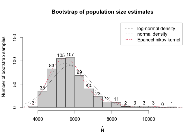
and information criteria support the second model:
#>  First model: AIC = 1736.854 BIC = 1759.01
#> Second model: AIC = 1734.803 BIC = 1756.959Work on this package is supported by the National Science Centre through OPUS 20 grant no. 2020/39/B/HS4/00941.
Chlebicki, P., & Beręsewicz, M. (2026). singleRcapture: An R Package for Single-Source Capture-Recapture Models. Journal of Statistical Software, 115(1), 1–30. https://doi.org/10.18637/jss.v115.i01
 @Article{,
    title = {{singleRcapture}: An {R} Package for Single-Source Capture-Recapture Models},
    author = {Piotr Chlebicki and Maciej Ber\c{e}sewicz},
    journal = {Journal of Statistical Software},
    year = {2025},
    volume = {115},
    number = {1},
    pages = {1--30},
    doi = {10.18637/jss.v115.i01},
  }