![]()
![]()
A stable version sentopics is available on CRAN:
install.packages("sentopics")The latest development version can be installed from GitHub:
devtools::install_github("odelmarcelle/sentopics") The development version requires the appropriate tools to compile C++ and Fortran source code.
Using a sample of press conferences from the European Central Bank,
an LDA model is easily created from a list of tokenized texts. See https://quanteda.io for
details on tokens input objects and pre-processing
functions.
library("sentopics")
print(ECB_press_conferences_tokens, 2)
# Tokens consisting of 3,860 documents and 5 docvars.
# 1_1 :
#  [1] "outcome"           "meeting"           "decision"
#  [4] ""                  "ecb"               "general"
#  [7] "council"           "governing_council" "executive"
# [10] "board"             "accordance"        "escb"
# [ ... and 7 more ]
#
# 1_2 :
#  [1] ""              "state"         "government"    "member"
#  [5] "executive"     "board"         "ecb"           "president"
#  [9] "vice"          "president"     "date"          "establishment"
# [ ... and 13 more ]
#
# [ reached max_ndoc ... 3,858 more documents ]
set.seed(123)
lda <- LDA(ECB_press_conferences_tokens, K = 3, alpha = .1)
lda <- fit(lda, 100)
lda
# An LDA model with 3 topics. Currently fitted by 100 Gibbs sampling iterations.
# ------------------Useful methods------------------
# fit       :Estimate the model using Gibbs sampling
# topics    :Return the most important topic of each document
# topWords  :Return a data.table with the top words of each topic/sentiment
# plot      :Plot a sunburst chart representing the estimated mixtures
# This message is displayed once per session, unless calling `print(x, extended = TRUE)`
There are various way to extract results from the model: it is either
possible to directly access the estimated mixtures from the
lda object or to use some helper functions.
# The document-topic distributions
head(lda$theta)
#       topic
# doc_id      topic1    topic2      topic3
#    1_1 0.005780347 0.9884393 0.005780347
#    1_2 0.004291845 0.9914163 0.004291845
#    1_3 0.015873016 0.9682540 0.015873016
#    1_4 0.009708738 0.9805825 0.009708738
#    1_5 0.008849558 0.9823009 0.008849558
#    1_6 0.006993007 0.9160839 0.076923077
# The document-topic in a 'long' format & optionally with meta-data
head(melt(lda, include_docvars = FALSE))
#     topic    .id        prob
#    <fctr> <char>       <num>
# 1: topic1    1_1 0.005780347
# 2: topic1    1_2 0.004291845
# 3: topic1    1_3 0.015873016
# 4: topic1    1_4 0.009708738
# 5: topic1    1_5 0.008849558
# 6: topic1    1_6 0.006993007
# The most probable words per topic
topWords(lda, output = "matrix")
#       topic1        topic2              topic3
#  [1,] "growth"      "governing_council" "euro_area"
#  [2,] "annual"      "fiscal"            "economic"
#  [3,] "rate"        "euro_area"         "growth"
#  [4,] "price"       "country"           "price"
#  [5,] "loan"        "growth"            "risk"
#  [6,] "monetary"    "policy"            "inflation"
#  [7,] "inflation"   "reform"            "development"
#  [8,] "euro_area"   "structural"        "price_stability"
#  [9,] "development" "market"            "quarter"
# [10,] "financial"   "bank"              "outlook"
Two visualization are also implemented: plot_topWords()
display the most probable words and plot() summarize the
topic proportions and their top words.
plot(lda)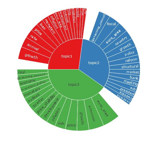
After properly incorporating date and sentiment metadata data (if
they are not already present in the tokens input), time
series functions allows to study the evolution of topic proportions and
related sentiment.
sentopics_date(lda)  |> head(2)
#       .id      .date
#    <char>     <Date>
# 1:    1_1 1998-06-09
# 2:    1_2 1998-06-09
sentopics_sentiment(lda) |> head(2)
#       .id  .sentiment
#    <char>       <num>
# 1:    1_1 -0.01470588
# 2:    1_2 -0.02500000
proportion_topics(lda, period = "month") |> head(2)
#                topic1    topic2     topic3
# 1998-06-01 0.04004786 0.9100265 0.04992568
# 1998-07-01 0.17387955 0.7276814 0.09843903
plot_sentiment_breakdown(lda, period = "quarter", rolling_window = 3)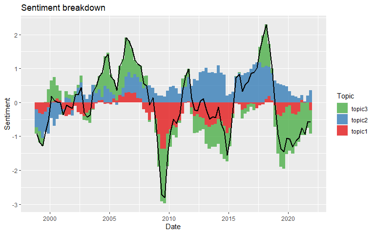
Feel free to refer to the vignettes of the package for a more extensive introduction to the features of the package. Because the package is not yet on CRAN, you’ll have to build the vignettes locally.
vignette("Basic_usage", package = "sentopics")
vignette("Topical_time_series", package = "sentopics")