![]()
Azka Ubaidillah, Ridson Al Farizal P
Ridson Al Farizal P <alfrzlp@gmail.com>
We designed this package to provide function for unit level of small
area estimation (Battese, Harter and Fuller model) using hierarchical
Bayesian (HB) method. It also provides datasets generated by data
generation (dummy_unit and dummy_area) and
real dataset (cornsoybean and
cornsoybeanmean). The rjags package is
employed to obtain parameter estimates
You can install the development version of saeHB.unit from GitHub with:
install.packages("devtools")
devtools::install_github("Alfrzlp/saeHB.unit")
Or you can install cran version with
install.packages(saeHB.unit)This is a basic example which shows you how to solve a common problem:
library(saeHB.unit)
library(ggplot2)
library(dplyr)
library(tidyr)
library(sae)

windowsFonts(
  poppins = windowsFont('poppins')
)glimpse(cornsoybean)
#> Rows: 37
#> Columns: 5
#> $ County <int> 1, 2, 3, 4, 4, 5, 5, 5, 6, 6, 6, 7, 7, 7, 8, 8, 8, 9, 9, 9…
#> $ CornHec <dbl> 165.76, 96.32, 76.08, 185.35, 116.43, 162.08, 152.04, 161.…
#> $ SoyBeansHec <dbl> 8.09, 106.03, 103.60, 6.47, 63.82, 43.50, 71.43, 42.49, 10…
#> $ CornPix <int> 374, 209, 253, 432, 367, 361, 288, 369, 206, 316, 145, 355…
#> $ SoyBeansPix <int> 55, 218, 250, 96, 178, 137, 206, 165, 218, 221, 338, 128, …
glimpse(cornsoybeanmeans)
#> Rows: 12
#> Columns: 6
#> $ CountyIndex <int> 1, 2, 3, 4, 5, 6, 7, 8, 9, 10, 11, 12
#> $ CountyName <fct> CerroGordo, Hamilton, Worth, Humboldt, Franklin,…
#> $ SampSegments <int> 1, 1, 1, 2, 3, 3, 3, 3, 4, 5, 5, 6
#> $ PopnSegments <dbl> 545, 566, 394, 424, 564, 570, 402, 567, 687, 569…
#> $ MeanCornPixPerSeg <dbl> 295.29, 300.40, 289.60, 290.74, 318.21, 257.17, …
#> $ MeanSoyBeansPixPerSeg <dbl> 189.70, 196.65, 205.28, 220.22, 188.06, 247.13, …Xarea <- cornsoybeanmeans %>%
dplyr::select(
County = CountyIndex,
CornPix = MeanCornPixPerSeg,
SoyBeansPix = MeanSoyBeansPixPerSeg
)
head(Xarea)
#> County CornPix SoyBeansPix
#> 1 1 295.29 189.70
#> 2 2 300.40 196.65
#> 3 3 289.60 205.28
#> 4 4 290.74 220.22
#> 5 5 318.21 188.06
#> 6 6 257.17 247.13Popn <- cornsoybeanmeans %>%
dplyr::select(CountyIndex, PopnSegments)
corn_eblup <- pbmseBHF(
CornHec ~ CornPix + SoyBeansPix,
dom = County,
meanxpop = Xarea, popnsize = Popn, data = cornsoybean, B = 50
)
#>
#> Bootstrap procedure with B = 50 iterations starts.
#> boundary (singular) fit: see help('isSingular')
#> b = 1
#> b = 2
#> boundary (singular) fit: see help('isSingular')
#> b = 3
#> b = 4
#> boundary (singular) fit: see help('isSingular')
#> b = 5
#> b = 6
#> b = 7
#> b = 8
#> b = 9
#> b = 10
#> boundary (singular) fit: see help('isSingular')
#> b = 11
#> b = 12
#> b = 13
#> boundary (singular) fit: see help('isSingular')
#> b = 14
#> b = 15
#> b = 16
#> boundary (singular) fit: see help('isSingular')
#> b = 17
#> boundary (singular) fit: see help('isSingular')
#> b = 18
#> b = 19
#> boundary (singular) fit: see help('isSingular')
#> b = 20
#> b = 21
#> b = 22
#> b = 23
#> b = 24
#> b = 25
#> b = 26
#> boundary (singular) fit: see help('isSingular')
#> b = 27
#> b = 28
#> b = 29
#> b = 30
#> b = 31
#> b = 32
#> boundary (singular) fit: see help('isSingular')
#> b = 33
#> boundary (singular) fit: see help('isSingular')
#> b = 34
#> b = 35
#> b = 36
#> b = 37
#> b = 38
#> b = 39
#> b = 40
#> boundary (singular) fit: see help('isSingular')
#> b = 41
#> b = 42
#> b = 43
#> b = 44
#> b = 45
#> b = 46
#> b = 47
#> b = 48
#> boundary (singular) fit: see help('isSingular')
#> b = 49
#> boundary (singular) fit: see help('isSingular')
#> b = 50
rse_eblup <- sqrt(corn_eblup$mse$mse) * 100 / corn_eblup$est$eblup$eblupcorn_hb <- hb_unit(
CornHec ~ SoyBeansPix + CornPix,
data_unit = cornsoybean,
data_area = Xarea,
domain = "County",
iter.update = 20
)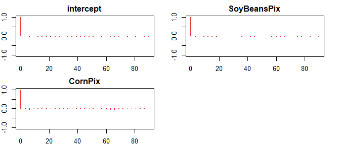
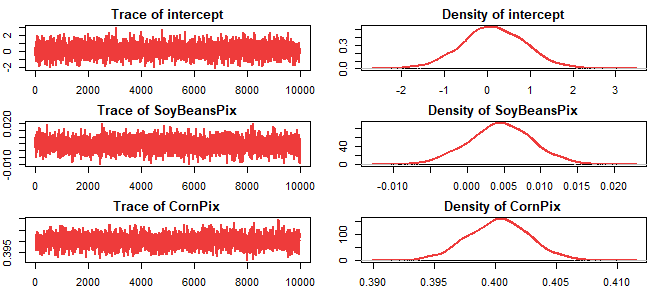
#>                   Mean         SD       2.5%        25%        50%        75%
#> intercept    0.1552265  0.7415844 -1.3078113 -0.3262636  0.1458748  0.6601395
#> SoyBeansPix  0.0045318  0.0044236 -0.0041645  0.0016640  0.0045969  0.0074832
#> CornPix      0.4002724  0.0025485  0.3951512  0.3985503  0.4002998  0.4019972
#>              97.5%
#> intercept   1.6317
#> SoyBeansPix 0.0132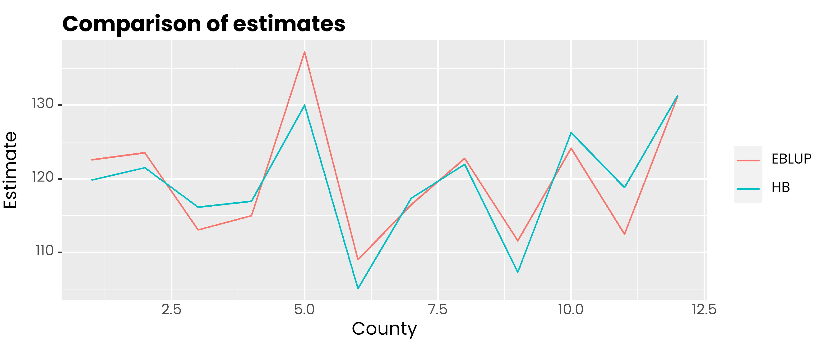
#> CornPix 0.4053data.frame(
id = 1:12,
hb = corn_hb$Est$MEAN,
eblup = corn_eblup$est$eblup$eblup
) %>%
pivot_longer(-1, names_to = "metode", values_to = "rse") %>%
ggplot(aes(x = id, y = rse, col = metode)) +
geom_line() +
scale_color_discrete(
labels = c('EBLUP', 'HB')
) +
labs(col = NULL, y = 'Estimate', x = 'County', title = 'Comparison of estimates') +
theme(
text = element_text(family = 'poppins'),
axis.ticks.x = element_blank(),
plot.title = element_text(face = 2, vjust = 0),
plot.subtitle = element_text(colour = 'gray30', vjust = 0)
)
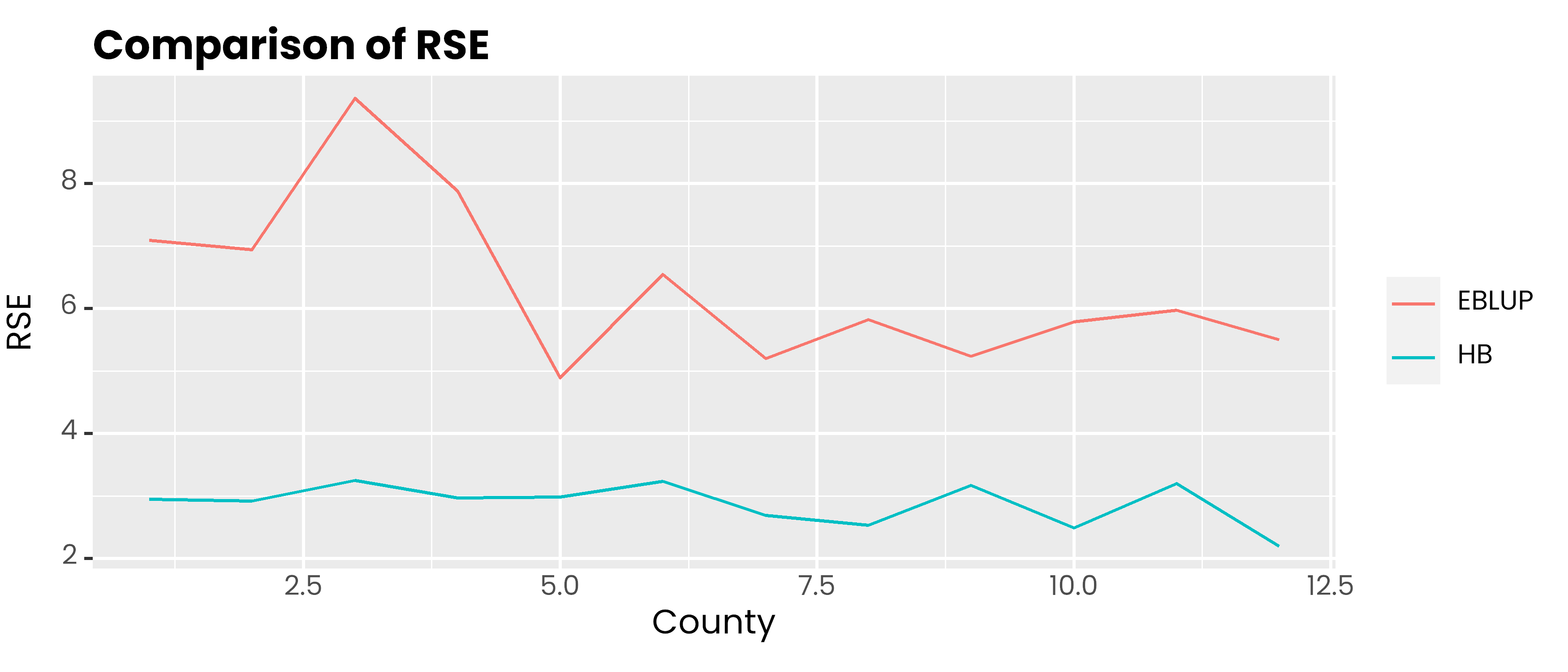
data.frame(
  id = 1:12,
  hb = corn_hb$Est$SD * 100 / corn_hb$Est$MEAN,
  eblup = rse_eblup
) %>%
  pivot_longer(-1, names_to = "metode", values_to = "rse") %>%
  ggplot(aes(x = id, y = rse, col = metode)) +
  geom_line() +
  scale_color_discrete(
    labels = c('EBLUP', 'HB')
  ) +
  labs(col = NULL, y = 'RSE', x = 'County', title = 'Comparison of RSE') +
  theme(
    text = element_text(family = 'poppins'),
    axis.ticks.x = element_blank(),
    plot.title = element_text(face = 2, vjust = 0),
    plot.subtitle = element_text(colour = 'gray30', vjust = 0)
  )
head(dummy_unit)
#>      domain     y_di       x1       x2
#> 181      d1 72.67585 13.88978 14.35716
#> 279      d1 63.10395 10.38460 13.58800
#> 343      d1 80.10076 16.36110 14.59864
#> 539      d1 68.83004 13.33046 14.17516
#> 670      d1 77.48515 18.62796 12.55454
#> 1424 d1 78.00826 13.44454 16.34891head(dummy_area)
#> domain x1 x2 parameter
#> 1 d1 15.05076 14.96766 77.03467
#> 2 d2 15.07153 14.98934 74.67858
#> 3 d3 14.96426 14.94145 73.35885
#> 4 d4 15.03803 15.02529 77.99655
#> 5 d5 14.98165 14.99815 76.76959
#> 6 d6 15.04244 15.00129 77.30116hb_model <- hb_unit(
formula = y_di ~ x1 + x2,
data_unit = dummy_unit,
data_area = dummy_area,
domain = "domain",
iter.update = 30,
plot = FALSE
)
#> Update 2/30 | ■■■ 7% | ETA: 2m Update 3/30 | ■■■■ 10% | ETA: 2m Update 4/30 | ■■■■■ 13% | ETA: 2m Update 5/30 | ■■■■■■ 17% | ETA: 3m Update 6/30 | ■■■■■■■ 20% | ETA: 3m Update 7/30 | ■■■■■■■■ 23% | ETA: 3m Update 8/30 | ■■■■■■■■■ 27% | ETA: 3m Update 9/30 | ■■■■■■■■■■ 30% | ETA: 3m Update 10/30 | ■■■■■■■■■■■ 33% | ETA: 3m Update 11/30 | ■■■■■■■■■■■■ 37% | ETA: 3m Update 12/30 | ■■■■■■■■■■■■■ 40% | ETA: 3m Update 13/30 | ■■■■■■■■■■■■■■ 43% | ETA: 3m Update 14/30 | ■■■■■■■■■■■■■■■ 47% | ETA: 3m Update 15/30 | ■■■■■■■■■■■■■■■■ 50% | ETA: 3m Update 16/30 | ■■■■■■■■■■■■■■■■■ 53% | ETA: 3m Update 17/30 | ■■■■■■■■■■■■■■■■■■ 57% | ETA: 2m Update 18/30 | ■■■■■■■■■■■■■■■■■■■ 60% | ETA: 2m Update 19/30 | ■■■■■■■■■■■■■■■■■■■■ 63% | ETA: 2m Update 20/30 | ■■■■■■■■■■■■■■■■■■■■■ 67% | ETA: 2m Update 21/30 | ■■■■■■■■■■■■■■■■■■■■■■ 70% | ETA: 2m Update 22/30 | ■■■■■■■■■■■■■■■■■■■■■■■ 73% | ETA: 2m Update 23/30 | ■■■■■■■■■■■■■■■■■■■■■■■■ 77% | ETA: 1m Update 24/30 | ■■■■■■■■■■■■■■■■■■■■■■■■■ 80% | ETA: 1m Update 25/30 | ■■■■■■■■■■■■■■■■■■■■■■■■■■ 83% | ETA: 1m Update 26/30 | ■■■■■■■■■■■■■■■■■■■■■■■■■■■ 87% | ETA: 46s Update 27/30 | ■■■■■■■■■■■■■■■■■■■■■■■■■■■■ 90% | ETA: 34s Update 28/30 | ■■■■■■■■■■■■■■■■■■■■■■■■■■■■■ 93% | ETA: 23s Update 29/30 | ■■■■■■■■■■■■■■■■■■■■■■■■■■■■■■ 97% | ETA: 11s
#> ── Coefficient ─────────────────────────────────────────────────────────────────
#> Mean SD 2.5% 25% 50% 75% 97.5%
#> intercept 0.3948102 0.0573688 0.2829102 0.3558277 0.3952609 0.4337828 0.5068
#> x1 2.0298812 0.0022426 2.0256112 2.0282862 2.0298828 2.0314088 2.0343
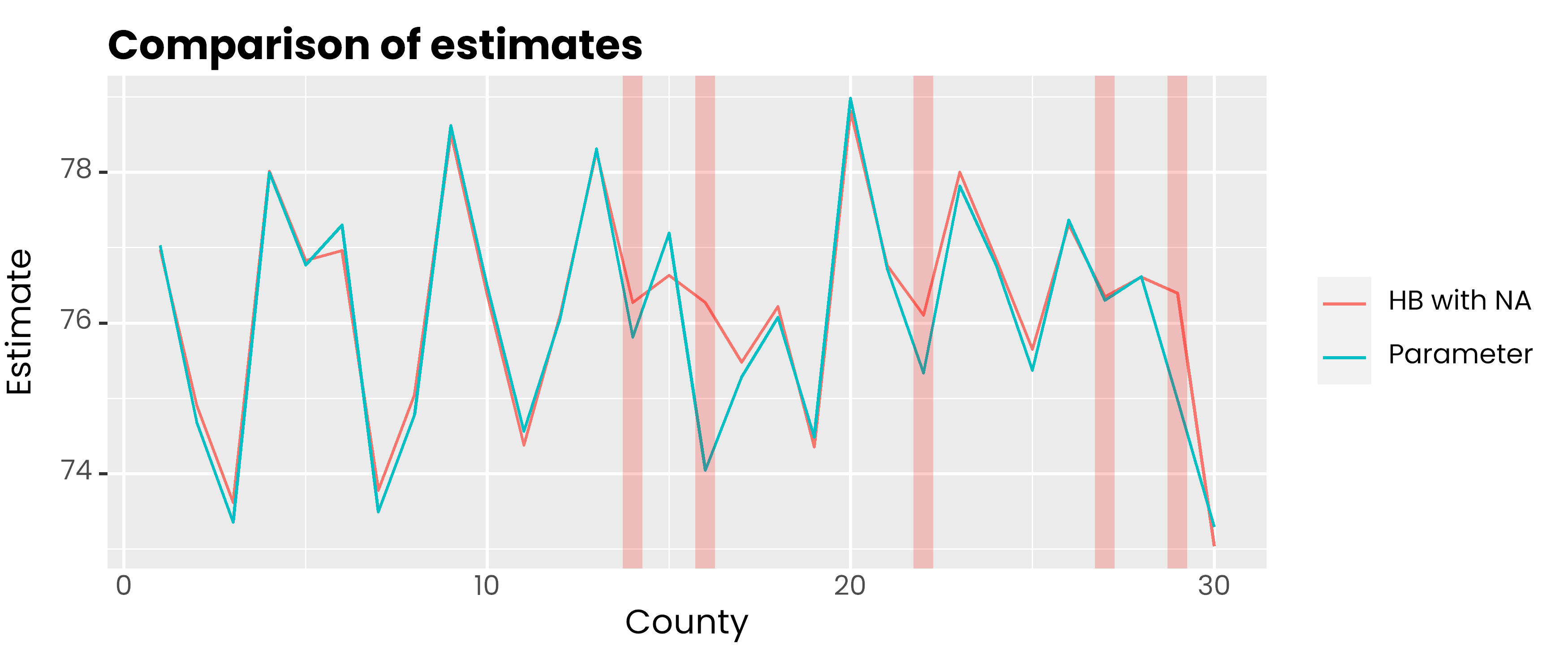
#> x2 3.0231039 0.0023648 3.0184731 3.0215362 3.0231553 3.0246763 3.0278This dataset contains NA in 5 domains out of 30 domains.
dummy_unit %>%
  dplyr::filter(is.na(y_di)) %>%
  sample_n(size = 5)
#>   domain y_di       x1       x2
#> 1    d22   NA 19.00794 11.30174
#> 2    d27   NA 19.09201 12.22442
#> 3    d27   NA 13.87459 13.50042
#> 4    d22   NA 12.26944 10.24241
#> 5    d27   NA 13.49637 11.45061
dummy_unit %>%
dplyr::filter(is.na(y_di)) %>%
distinct(domain)
#> domain
#> 1 d14
#> 2 d16
#> 3 d22
#> 4 d27
#> 5 d29saeHB.unit::autoplot(hb_model)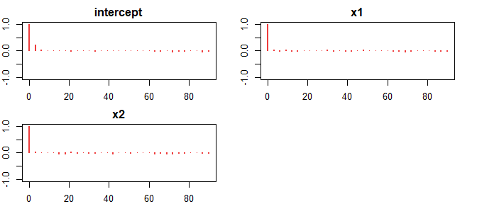
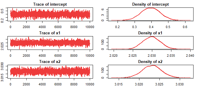
summary(hb_model)
#>                Mean        SD      2.5%       25%       50%       75%  97.5%
#> intercept 0.3948102 0.0573688 0.2829102 0.3558277 0.3952609 0.4337828 0.5068
#> x1        2.0298812 0.0022426 2.0256112 2.0282862 2.0298828 2.0314088 2.0343
#> x2 3.0231039 0.0023648 3.0184731 3.0215362 3.0231553 3.0246763 3.0278data.frame(
id = 1:30,
hb = hb_model$Est$MEAN,
parameter = dummy_area$parameter
) %>%
pivot_longer(-1, names_to = "metode", values_to = "rse") %>%
ggplot(aes(x = id, y = rse, col = metode)) +
geom_line() +
geom_vline(xintercept = c(14, 16, 22, 27, 29), color = 'red', alpha = 0.2, lwd = 3) +
scale_color_discrete(
labels = c('HB with NA', 'Parameter')
) +
labs(col = NULL, y = 'Estimate', x = 'County', title = 'Comparison of estimates') +
theme(
text = element_text(family = 'poppins'),
axis.ticks.x = element_blank(),
plot.title = element_text(face = 2, vjust = 0),
plot.subtitle = element_text(colour = 'gray30', vjust = 0)
)
Battese, G. E., Harter, R. M., & Fuller, W. A. (1988). An error-components model for prediction of county crop areas using survey and satellite data. Journal of the American Statistical Association, 83(401), 28-36.
Rao, J. N., & Molina, I. (2015). Small area estimation. John Wiley & Sons.