15 January, 2021
assess_reference_loo()
This is an R package for performing genetic stock identification (GSI) and associated tasks. Additionally, it includes a method designed to diagnose and correct a bias recently documented in genetic stock identification. The bias occurs when mixture proportion estimates are desired for groups of populations (reporting units) and the number of populations within each reporting unit are uneven.
In order to run C++ implementations of MCMC, rubias requires the package Rcpp (and now, also, RcppParallel for the baseline resampling option), which in turn requires an Rtools installation (if you are on Windows) or XCode (if you are on a Mac). After cloning into the repository with the above dependencies installed, build & reload the package to view further documentation.
The script “/R-main/coalescent_sim” was used to generate coalescent
simulations for bias correction validation. This is unnecessary for
testing the applicability of our methods to any particular dataset,
which should be done using assess_reference_loo() and
assess_pb_bias_correction(). coalescent_sim()
creates simulated populations using the ms coalescent
simulation program, available from the Hudson lab at UChicago, and the
GSImulator and ms2geno packages, available at
https://github.com/eriqande, and so requires more
dependencies than the rest of the package.
The functions for conducting genetic mixture analysis and for doing simulation assessment to predict the accuracy of a set of genetic markers for genetic stock identification require that genetic data be input as a data frame in a specific format:
sample_type: a column telling whether the sample is a
reference sample or a mixture sample.repunit: the reporting unit that an
individual/collection belongs to. This is required if sample_type is
reference. And if sample_type is mixture then
repunit must be NA.collection: for reference samples, the name of the
population that the individual is from. For mixture samples, this is the
name of the particular sample (i.e. stratum or port that is to be
treated together in space and time). This must be a character, not a
factor.indiv a character vector with the ID of the fish. These
must be unique.rubias, we intended to allow
both the repunit and the collection columns to
be either character vectors or factors. Having them as factors might be
desirable if, for example, a certain sort order of the collections or
repunits was desired. However at some point it became clear to
Eric that, given our approach to converting all the data to a C++ data
structure of integers, for rapid analyis, we would be exposing ourselves
to greater opportunities for bugginess by allowing repunit
and collection to be factors. Accordingly, they
must be character vectors. If they are not,
rubias will throw an error. Note: if you
do have a specific sort order for your collections or repunits, you can
always change them into factors after analysis with rubias.
Additionally, you can keep extra columns in your original data frame
(for example repunit_f or collection_f) in
which the repunits or the collections are stored as factors. See, for
example the data file alewife. Or you can just keep a
character vector that has the sort order you would like, so as to use it
when changing things to factors after rubias analysis.
(See, for instance, chinook_repunit_levels.)At the request of the good folks at ADFG, I introduced a few hacks to
allow the input to include markers that are haploid (for example mtDNA
haplotypes). To denote a marker as haploid you still give it two
columns of data in your data frame, but the second column of the
haploid marker must be entirely NAs. When rubias is
processing the data and it sees this, it assumes that the marker is
haploid and it treats it appropriately.
Note that if you have a diploid marker it typically does not make sense to mark one of the gene copies as missing and the other as non-missing. Accordingly, if you have a diploid marker that records just one of the gene copies as missing in any individual, it is going to throw an error. Likewise, if your haploid marker does not have every single individual with and NA at the second gene copy, then it’s also going to throw an error.
Here are the meta data columns and the first two loci for eight
individuals in the chinook reference data set that comes
with the package:
library(tidyverse)  # load up the tidyverse library, we will use it later...
#> ── Attaching packages ─────────────────────────────────────── tidyverse 1.3.0 ──
#> ✓ ggplot2 3.3.2     ✓ purrr   0.3.4
#> ✓ tibble  3.0.4     ✓ dplyr   1.0.2
#> ✓ tidyr   1.1.2     ✓ stringr 1.4.0
#> ✓ readr   1.4.0     ✓ forcats 0.5.0
#> ── Conflicts ────────────────────────────────────────── tidyverse_conflicts() ──
#> x dplyr::filter() masks stats::filter()
#> x dplyr::lag()    masks stats::lag()
library(rubias)
head(chinook[, 1:8])
#> # A tibble: 6 x 8
#>   sample_type repunit collection indiv Ots_94857.232 Ots_94857.232.1
#>   <chr>       <chr>   <chr>      <chr>         <int>           <int>
#> 1 reference   Centra… Feather_H… Feat…             2               2
#> 2 reference   Centra… Feather_H… Feat…             2               4
#> 3 reference   Centra… Feather_H… Feat…             2               4
#> 4 reference   Centra… Feather_H… Feat…             2               4
#> 5 reference   Centra… Feather_H… Feat…             2               2
#> 6 reference   Centra… Feather_H… Feat…             2               4
#> # … with 2 more variables: Ots_102213.210 <int>, Ots_102213.210.1 <int>Here is the same for the mixture data frame that goes along with that reference data set:
head(chinook_mix[, 1:8])
#> # A tibble: 6 x 8
#>   sample_type repunit collection indiv Ots_94857.232 Ots_94857.232.1
#>   <chr>       <chr>   <chr>      <chr>         <int>           <int>
#> 1 mixture     <NA>    rec2       T124…             4               2
#> 2 mixture     <NA>    rec2       T124…             4               2
#> 3 mixture     <NA>    rec2       T124…             4               4
#> 4 mixture     <NA>    rec1       T124…             4               4
#> 5 mixture     <NA>    rec1       T124…             2               2
#> 6 mixture     <NA>    rec1       T124…             4               2
#> # … with 2 more variables: Ots_102213.210 <int>, Ots_102213.210.1 <int>Sometimes, for a variety of reasons, an individual’s genotype might
appear more than once in a data set. rubias has a quick and
dirty function to spot pairs of individuals that share a large number of
genotypes. Clearly you only want to look at pairs that don’t have a
whole lot of missing data, so one parameter is the fraction of loci that
are non-missing in either fish. In our experience with Fluidigm assays,
if a fish is missing at > 10% of the SNPs, the remaining genotypes
are likely to have a fairly high error rate. So, to look for matching
samples, let’s require 85% of the genotypes to be non-missing in both
members of the pair. The last parameter is the fraction of non-missing
loci at which the pair has the same genotype. We will set that to 0.94
first. Here we see it in action:
# combine chinook and chinook_mix into one big data frame,
# but drop the California_Coho collection because Coho all
# have pretty much the same genotype at these loci!
chinook_all <- bind_rows(chinook, chinook_mix) %>%
  filter(collection != "California_Coho")

# then toss them into a function.  This takes half a minute or so...
matchy_pairs <- close_matching_samples(D = chinook_all,
                                       gen_start_col = 5,
                                       min_frac_non_miss = 0.85,
                                       min_frac_matching = 0.94
                                       )
#> Summary Statistics:
#>
#> 9510 Individuals in Sample
#>
#> 91 Loci: AldB1.122, AldoB4.183, OTNAML12_1.SNP1, Ots_100884.287, Ots_101119.381, Ots_101704.143, Ots_102213.210, Ots_102414.395, Ots_102420.494, Ots_102457.132, Ots_102801.308, Ots_102867.609, Ots_103041.52, Ots_104063.132, Ots_104569.86, Ots_105105.613, Ots_105132.200, Ots_105401.325, Ots_105407.117, Ots_106499.70, Ots_106747.239, Ots_107074.284, Ots_107285.93, Ots_107806.821, Ots_108007.208, Ots_108390.329, Ots_108735.302, Ots_109693.392, Ots_110064.383, Ots_110201.363, Ots_110495.380, Ots_110551.64, Ots_111312.435, Ots_111666.408, Ots_111681.657, Ots_112301.43, Ots_112419.131, Ots_112820.284, Ots_112876.371, Ots_113242.216, Ots_113457.40, Ots_117043.255, Ots_117242.136, Ots_117432.409, Ots_118175.479, Ots_118205.61, Ots_118938.325, Ots_122414.56, Ots_123048.521, Ots_123921.111, Ots_124774.477, Ots_127236.62, Ots_128302.57, Ots_128693.461, Ots_128757.61, Ots_129144.472, Ots_129170.683, Ots_129458.451, Ots_130720.99, Ots_131460.584, Ots_131906.141, Ots_94857.232, Ots_96222.525, Ots_96500.180, Ots_97077.179, Ots_99550.204, Ots_ARNT.195, Ots_AsnRS.60, Ots_aspat.196, Ots_CD59.2, Ots_CD63, Ots_EP.529, Ots_GDH.81x, Ots_HSP90B.385, Ots_MHC1, Ots_mybp.85, Ots_myoD.364, Ots_Ots311.101x, Ots_PGK.54, Ots_Prl2, Ots_RFC2.558, Ots_SClkF2R2.135, Ots_SWS1op.182, Ots_TAPBP, Ots_u07.07.161, Ots_u07.49.290, Ots_u4.92, OTSBMP.2.SNP1, OTSTF1.SNP1, S71.336, unk_526
#>
#> 39 Reporting Units: CentralValleyfa, CentralValleysp, CentralValleywi, CaliforniaCoast, KlamathR, NCaliforniaSOregonCoast, RogueR, MidOregonCoast, NOregonCoast, WillametteR, DeschutesRfa, LColumbiaRfa, LColumbiaRsp, MidColumbiaRtule, UColumbiaRsufa, MidandUpperColumbiaRsp, SnakeRfa, SnakeRspsu, NPugetSound, WashingtonCoast, SPugetSound, LFraserR, LThompsonR, EVancouverIs, WVancouverIs, MSkeenaR, MidSkeenaR, LSkeenaR, SSEAlaska, NGulfCoastAlsekR, NGulfCoastKarlukR, TakuR, NSEAlaskaChilkatR, NGulfCoastSitukR, CopperR, SusitnaR, LKuskokwimBristolBay, MidYukon
#>
#> 68 Collections: Feather_H_sp, Butte_Cr_Sp, Mill_Cr_sp, Deer_Cr_sp, UpperSacramento_R_sp, Feather_H_fa, Butte_Cr_fa, Mill_Cr_fa, Deer_Cr_fa, Mokelumne_R_fa, Battle_Cr, Sacramento_R_lf, Sacramento_H, Eel_R, Russian_R, Klamath_IGH_fa, Trinity_H_sp, Smith_R, Chetco_R, Cole_Rivers_H, Applegate_Cr, Coquille_R, Umpqua_sp, Nestucca_H, Siuslaw_R, Alsea_R, Nehalem_R, Siletz_R, N_Santiam_H, McKenzie_H, L_Deschutes_R, Cowlitz_H_fa, Cowlitz_H_sp, Kalama_H_sp, Spring_Cr_H, Hanford_Reach, PriestRapids_H, Wells_H, Wenatchee_R, CleElum, Lyons_Ferry_H, Rapid_R_H, McCall_H, Kendall_H_sp, Forks_Cr_H, Soos_H, Marblemount_H_sp, QuinaltLake_f, Harris_R, Birkenhead_H, Spius_H, Big_Qual_H, Robertson_H, Morice_R, Kitwanga_R, L_Kalum_R, LPW_Unuk_R, Goat_Cr, Karluk_R, LittleTatsamenie, Tahini_R, Situk_R, Sinona_Ck, Montana_Ck, George_R, Kanektok_R, Togiak_R, Kantishna_R
#>
#> 3.85% of allelic data identified as missing

# see that that looks like:
matchy_pairs %>%
  arrange(desc(num_non_miss), desc(num_match))
#> # A tibble: 33 x 10
#>    num_non_miss num_match indiv_1 indiv_2 collection_1 collection_2
#>           <int>     <int> <chr>   <chr>   <chr>        <chr>
#>  1           91        91 T124864 T124866 rec3         rec1
#>  2           91        91 T124864 T125335 rec3         rec3
#>  3           91        91 T124866 T125335 rec1         rec3
#>  4           91        91 T126402 T126403 rec2         rec2
#>  5           91        90 Mill_C… Mill_C… Mill_Cr_sp   Mill_Cr_sp
#>  6           91        90 Cole_R… Cole_R… Cole_Rivers… Cole_Rivers…
#>  7           91        90 Cole_R… Cole_R… Cole_Rivers… Cole_Rivers…
#>  8           91        90 Umpqua… Umpqua… Umpqua_sp    Umpqua_sp
#>  9           91        90 Umpqua… Umpqua… Umpqua_sp    Umpqua_sp
#> 10           91        90 T125044 T125337 rec2         rec1
#> # … with 23 more rows, and 4 more variables: sample_type_1 <chr>,
#> #   repunit_1 <chr>, sample_type_2 <chr>, repunit_2 <chr>
Check that out. This reveals 33 pairs in the data set that are likely duplicate samples.
If we reduce the min_frac_matching, we get more matches, but these are very unlikely to be the same individual, unless genotyping error rates are very high.
# then toss them into a function.  This takes half a minute or so...
matchy_pairs2 <- close_matching_samples(D = chinook_all,
                                       gen_start_col = 5,
                                       min_frac_non_miss = 0.85,
                                       min_frac_matching = 0.85
                                       )
#> Summary Statistics:
#>
#> 9510 Individuals in Sample
#>
#> 91 Loci: AldB1.122, AldoB4.183, OTNAML12_1.SNP1, Ots_100884.287, Ots_101119.381, Ots_101704.143, Ots_102213.210, Ots_102414.395, Ots_102420.494, Ots_102457.132, Ots_102801.308, Ots_102867.609, Ots_103041.52, Ots_104063.132, Ots_104569.86, Ots_105105.613, Ots_105132.200, Ots_105401.325, Ots_105407.117, Ots_106499.70, Ots_106747.239, Ots_107074.284, Ots_107285.93, Ots_107806.821, Ots_108007.208, Ots_108390.329, Ots_108735.302, Ots_109693.392, Ots_110064.383, Ots_110201.363, Ots_110495.380, Ots_110551.64, Ots_111312.435, Ots_111666.408, Ots_111681.657, Ots_112301.43, Ots_112419.131, Ots_112820.284, Ots_112876.371, Ots_113242.216, Ots_113457.40, Ots_117043.255, Ots_117242.136, Ots_117432.409, Ots_118175.479, Ots_118205.61, Ots_118938.325, Ots_122414.56, Ots_123048.521, Ots_123921.111, Ots_124774.477, Ots_127236.62, Ots_128302.57, Ots_128693.461, Ots_128757.61, Ots_129144.472, Ots_129170.683, Ots_129458.451, Ots_130720.99, Ots_131460.584, Ots_131906.141, Ots_94857.232, Ots_96222.525, Ots_96500.180, Ots_97077.179, Ots_99550.204, Ots_ARNT.195, Ots_AsnRS.60, Ots_aspat.196, Ots_CD59.2, Ots_CD63, Ots_EP.529, Ots_GDH.81x, Ots_HSP90B.385, Ots_MHC1, Ots_mybp.85, Ots_myoD.364, Ots_Ots311.101x, Ots_PGK.54, Ots_Prl2, Ots_RFC2.558, Ots_SClkF2R2.135, Ots_SWS1op.182, Ots_TAPBP, Ots_u07.07.161, Ots_u07.49.290, Ots_u4.92, OTSBMP.2.SNP1, OTSTF1.SNP1, S71.336, unk_526
#>
#> 39 Reporting Units: CentralValleyfa, CentralValleysp, CentralValleywi, CaliforniaCoast, KlamathR, NCaliforniaSOregonCoast, RogueR, MidOregonCoast, NOregonCoast, WillametteR, DeschutesRfa, LColumbiaRfa, LColumbiaRsp, MidColumbiaRtule, UColumbiaRsufa, MidandUpperColumbiaRsp, SnakeRfa, SnakeRspsu, NPugetSound, WashingtonCoast, SPugetSound, LFraserR, LThompsonR, EVancouverIs, WVancouverIs, MSkeenaR, MidSkeenaR, LSkeenaR, SSEAlaska, NGulfCoastAlsekR, NGulfCoastKarlukR, TakuR, NSEAlaskaChilkatR, NGulfCoastSitukR, CopperR, SusitnaR, LKuskokwimBristolBay, MidYukon
#>
#> 68 Collections: Feather_H_sp, Butte_Cr_Sp, Mill_Cr_sp, Deer_Cr_sp, UpperSacramento_R_sp, Feather_H_fa, Butte_Cr_fa, Mill_Cr_fa, Deer_Cr_fa, Mokelumne_R_fa, Battle_Cr, Sacramento_R_lf, Sacramento_H, Eel_R, Russian_R, Klamath_IGH_fa, Trinity_H_sp, Smith_R, Chetco_R, Cole_Rivers_H, Applegate_Cr, Coquille_R, Umpqua_sp, Nestucca_H, Siuslaw_R, Alsea_R, Nehalem_R, Siletz_R, N_Santiam_H, McKenzie_H, L_Deschutes_R, Cowlitz_H_fa, Cowlitz_H_sp, Kalama_H_sp, Spring_Cr_H, Hanford_Reach, PriestRapids_H, Wells_H, Wenatchee_R, CleElum, Lyons_Ferry_H, Rapid_R_H, McCall_H, Kendall_H_sp, Forks_Cr_H, Soos_H, Marblemount_H_sp, QuinaltLake_f, Harris_R, Birkenhead_H, Spius_H, Big_Qual_H, Robertson_H, Morice_R, Kitwanga_R, L_Kalum_R, LPW_Unuk_R, Goat_Cr, Karluk_R, LittleTatsamenie, Tahini_R, Situk_R, Sinona_Ck, Montana_Ck, George_R, Kanektok_R, Togiak_R, Kantishna_R
#>
#> 3.85% of allelic data identified as missing

# see that that looks like:
matchy_pairs2 %>%
  arrange(desc(num_non_miss), desc(num_match))
#> # A tibble: 46 x 10
#>    num_non_miss num_match indiv_1 indiv_2 collection_1 collection_2
#>           <int>     <int> <chr>   <chr>   <chr>        <chr>
#>  1           91        91 T124864 T124866 rec3         rec1
#>  2           91        91 T124864 T125335 rec3         rec3
#>  3           91        91 T124866 T125335 rec1         rec3
#>  4           91        91 T126402 T126403 rec2         rec2
#>  5           91        90 Mill_C… Mill_C… Mill_Cr_sp   Mill_Cr_sp
#>  6           91        90 Cole_R… Cole_R… Cole_Rivers… Cole_Rivers…
#>  7           91        90 Cole_R… Cole_R… Cole_Rivers… Cole_Rivers…
#>  8           91        90 Umpqua… Umpqua… Umpqua_sp    Umpqua_sp
#>  9           91        90 Umpqua… Umpqua… Umpqua_sp    Umpqua_sp
#> 10           91        90 T125044 T125337 rec2         rec1
#> # … with 36 more rows, and 4 more variables: sample_type_1 <chr>,
#> #   repunit_1 <chr>, sample_type_2 <chr>, repunit_2 <chr>
A more principled approach would be to use the allele frequencies in each collection and take a likelihood based approach, but this is adequate for finding obvious duplicates.
In some cases, you might know (more or less unambiguously) the origin of some fish in a particular mixture sample. For example, if 10% of the individuals in a mixture carried coded wire tags, then you would want to include them in the sample, but make sure that their collections of origin were hard-coded to be what the CWTs said. Another scenario in which this might occur is when the genetic data were used for parentage-based tagging of the individuals in the mixture sample. In that case, some individuals might be placed with very high confidence to parents. Then, they should be included in the mixture as having come from a known collection. The folks at the DFO in Nanaimo, Canada are doing an amazing job with PBT and wondered if rubias could be modified to deal with the latter situation.
We’ve made some small additions to accommodate this. rubias does not
do any actual inference of parentage, but if you know the origin of some
fish in the mixture, that can be included in the rubias analysis. The
way you do this with the function infer_mixture() is to
include a column called known_collection in both the
reference data frame and the mixture data frame. In the reference data
frame, known_collection should just be a copy of the
collection column. However, in the mixture data frame each
entry in known_collection should be the collection that the
individual is known to be from (i.e. using parentage inference or a
CWT), or, if the individual is not known to be from any collection, it
should be NA. Note that the names of the collections in
known_collection must match those found in the
collection column in the reference data set.
These modifications are not allowed for the parametric bootstrap (PB)
method in infer_mixture().
This is done with the infer_mixture function. In the
example data chinook_mix our data consist of fish caught in
three different fisheries, rec1, rec2, and
rec3 as denoted in the collection column. Each of those
collections is treated as a separate sample, getting its own mixing
proportion estimate. This is how it is run with the default options:
mix_est <- infer_mixture(reference = chinook,
                         mixture = chinook_mix,
                         gen_start_col = 5)
#> Collating data; compiling reference allele frequencies, etc.   time: 1.64 seconds
#> Computing reference locus specific means and variances for computing mixture z-scores   time: 0.24 seconds
#> Working on mixture collection: rec2 with 772 individuals
#>   calculating log-likelihoods of the mixture individuals.   time: 0.12 seconds
#>   performing 2000 total sweeps, 100 of which are burn-in and will not be used in computing averages in method "MCMC"   time: 0.63 seconds
#>   tidying output into a tibble.   time: 0.25 seconds
#> Working on mixture collection: rec1 with 743 individuals
#>   calculating log-likelihoods of the mixture individuals.   time: 0.11 seconds
#>   performing 2000 total sweeps, 100 of which are burn-in and will not be used in computing averages in method "MCMC"   time: 0.61 seconds
#>   tidying output into a tibble.   time: 0.26 seconds
#> Working on mixture collection: rec3 with 741 individuals
#>   calculating log-likelihoods of the mixture individuals.   time: 0.11 seconds
#>   performing 2000 total sweeps, 100 of which are burn-in and will not be used in computing averages in method "MCMC"   time: 0.60 seconds
#>   tidying output into a tibble.   time: 0.29 seconds
The result comes back as a list of four tidy data frames:
mixing_proportions: the mixing proportions. The column
pi holds the estimated mixing proportion for each
collection.indiv_posteriors: this holds, for each individual, the
posterior means of group membership in each collection. Column
PofZ holds those values. Column log_likelihood
holds the log of the probability of the individuals genotype given it is
from the collection. Also included are n_non_miss_loci and
n_miss_loci which are the number of observed loci and the
number of missing loci at the individual. A list column
missing_loci contains vectors with the indices (and the
names) of the loci that are missing in that individual. It also includes
a column z_score which can be used to diagnose fish that
don’t belong to any samples in the reference data base (see below).mix_prop_traces: MCMC traces of the mixing proportions
for each collection. You will use these if you want to make density
estimates of the posterior distribution of the mixing proportions or if
you want to compute credible intervals.bootstrapped_proportions: This is NULL in the above
example, but if we had chosen method = "PB" then this would
be a tibble of bootstrap-corrected reporting unit mixing
proportions.These data frames look like this:
lapply(mix_est, head)
#> $mixing_proportions
#> # A tibble: 6 x 4
#>   mixture_collection repunit         collection                  pi
#>   <chr>              <chr>           <chr>                    <dbl>
#> 1 rec2               CentralValleyfa Feather_H_sp         0.0781
#> 2 rec2               CentralValleysp Butte_Cr_Sp          0.0000448
#> 3 rec2               CentralValleysp Mill_Cr_sp           0.0000457
#> 4 rec2               CentralValleysp Deer_Cr_sp           0.0000509
#> 5 rec2               CentralValleysp UpperSacramento_R_sp 0.000310
#> 6 rec2               CentralValleyfa Feather_H_fa         0.153
#>
#> $indiv_posteriors
#> # A tibble: 6 x 10
#>   mixture_collect… indiv repunit collection     PofZ log_likelihood z_score
#>   <chr>            <chr> <chr>   <chr>         <dbl>          <dbl>   <dbl>
#> 1 rec2             T124… Centra… Feather_H… 1.80e-28          -137.   -13.1
#> 2 rec2             T124… Centra… Feather_H… 1.01e-27          -136.   -12.6
#> 3 rec2             T124… Centra… Butte_Cr_… 1.57e-24          -130.   -10.5
#> 4 rec2             T124… Centra… Mill_Cr_fa 6.76e-30          -135.   -11.8
#> 5 rec2             T124… Centra… Deer_Cr_fa 1.49e-28          -134.   -11.6
#> 6 rec2             T124… Centra… Mokelumne… 1.91e-27          -134.   -12.3
#> # … with 3 more variables: n_non_miss_loci <int>, n_miss_loci <int>,
#> #   missing_loci <list>
#>
#> $mix_prop_traces
#> # A tibble: 6 x 5
#>   mixture_collection sweep repunit         collection               pi
#>   <chr>              <int> <chr>           <chr>                 <dbl>
#> 1 rec2                   0 CentralValleyfa Feather_H_sp         0.0145
#> 2 rec2                   0 CentralValleysp Butte_Cr_Sp          0.0145
#> 3 rec2                   0 CentralValleysp Mill_Cr_sp           0.0145
#> 4 rec2                   0 CentralValleysp Deer_Cr_sp           0.0145
#> 5 rec2                   0 CentralValleysp UpperSacramento_R_sp 0.0145
#> 6 rec2                   0 CentralValleyfa Feather_H_fa         0.0145
#>
#> $bootstrapped_proportions
#> # A tibble: 0 x 0In some cases there might be a reason to explicitly set the
parameters of the Dirichlet prior on the mixing proportions of the
collections. For a contrived example, we could imagine that we wanted a
Dirichlet prior with all parameters equal to 1/(# of collections),
except for the parameters for all the Central Valley Fall Run
populations, to which we would like to assign Dirichlet parameters of 2.
That can be accomplished with the pi_prior argument to the
infer_mixture() function, which will let you pass in a
tibble in which one column named “collection” gives the collection, and
the other column, named “pi_param” gives the desired parameter.
Here we construct that kind of input:
prior_tibble <- chinook %>%
  count(repunit, collection) %>%
  filter(repunit == "CentralValleyfa") %>%
  select(collection) %>%
  mutate(pi_param = 2)

# see what it looks like:
prior_tibble
#> # A tibble: 8 x 2
#>   collection      pi_param
#>   <chr>              <dbl>
#> 1 Battle_Cr              2
#> 2 Butte_Cr_fa            2
#> 3 Deer_Cr_fa             2
#> 4 Feather_H_fa           2
#> 5 Feather_H_sp           2
#> 6 Mill_Cr_fa             2
#> 7 Mokelumne_R_fa         2
#> 8 Sacramento_R_lf        2
Then we can run that in infer_mixture():
set.seed(12)
mix_est_with_prior <- infer_mixture(reference = chinook,
                         mixture = chinook_mix,
                         gen_start_col = 5,
                         pi_prior = prior_tibble)
#> Collating data; compiling reference allele frequencies, etc.   time: 1.56 seconds
#> Computing reference locus specific means and variances for computing mixture z-scores   time: 0.24 seconds
#> Working on mixture collection: rec2 with 772 individuals
#> Joining, by = "collection"
#>   calculating log-likelihoods of the mixture individuals.   time: 0.12 seconds
#>   performing 2000 total sweeps, 100 of which are burn-in and will not be used in computing averages in method "MCMC"   time: 0.62 seconds
#>   tidying output into a tibble.   time: 0.25 seconds
#> Working on mixture collection: rec1 with 743 individuals
#> Joining, by = "collection"
#>   calculating log-likelihoods of the mixture individuals.   time: 0.11 seconds
#>   performing 2000 total sweeps, 100 of which are burn-in and will not be used in computing averages in method "MCMC"   time: 0.61 seconds
#>   tidying output into a tibble.   time: 0.27 seconds
#> Working on mixture collection: rec3 with 741 individuals
#> Joining, by = "collection"
#>   calculating log-likelihoods of the mixture individuals.   time: 0.11 seconds
#>   performing 2000 total sweeps, 100 of which are burn-in and will not be used in computing averages in method "MCMC"   time: 0.59 seconds
#>   tidying output into a tibble.   time: 0.28 seconds
and now, for fun, we can compare the results for the mixing proportions of different collections there with and without the prior for the mixture collection rec1:
comp_mix_ests <- list(
  `pi (default prior)` = mix_est$mixing_proportions,
  `pi (cv fall gets 2s prior)` = mix_est_with_prior$mixing_proportions
) %>%
  bind_rows(.id = "prior_type") %>%
  filter(mixture_collection == "rec1") %>%
  select(prior_type, repunit, collection, pi) %>%
  spread(prior_type, pi) %>%
  mutate(coll_group = ifelse(repunit == "CentralValleyfa", "CV_fall", "Not_CV_fall"))

ggplot(comp_mix_ests,
       aes(x = `pi (default prior)`,
           y = `pi (cv fall gets 2s prior)`,
           colour = coll_group
           )) +
  geom_point() +
  geom_abline(slope = 1, intercept = 0, linetype = "dashed")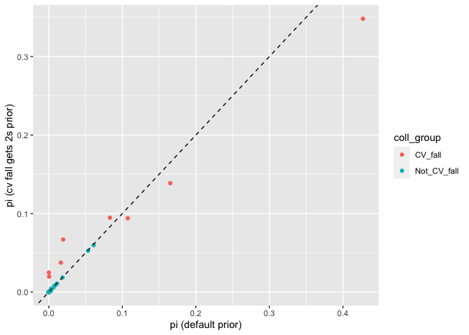
Yep, slightly different than before. Let’s look at the sums of everything:
comp_mix_ests %>%
  group_by(coll_group) %>%
  summarise(with_explicit_prior = sum(`pi (cv fall gets 2s prior)`),
            with_default_prior = sum(`pi (default prior)`))
#> `summarise()` ungrouping output (override with `.groups` argument)
#> # A tibble: 2 x 3
#>   coll_group  with_explicit_prior with_default_prior
#>   <chr>                     <dbl>              <dbl>
#> 1 CV_fall                   0.824              0.819
#> 2 Not_CV_fall               0.176              0.181
We see that for the most part this change to the prior changed the distribution of fish into different collections within the Central Valley Fall reporting unit. This is not suprising—it is very hard to tell apart fish from those different collections. However, it did not greatly change the estimated proportion of the whole reporting unit. This also turns out to make sense if you consider the effect that the extra weight in the prior will have.
This is a simple operation in the tidyverse:
# for mixing proportions
rep_mix_ests <- mix_est$mixing_proportions %>%
  group_by(mixture_collection, repunit) %>%
  summarise(repprop = sum(pi))  # adding mixing proportions over collections in the repunit
#> `summarise()` regrouping output by 'mixture_collection' (override with `.groups` argument)

# for individuals posteriors
rep_indiv_ests <- mix_est$indiv_posteriors %>%
  group_by(mixture_collection, indiv, repunit) %>%
  summarise(rep_pofz = sum(PofZ))
#> `summarise()` regrouping output by 'mixture_collection', 'indiv' (override with `.groups` argument)The full MCMC output for the mixing proportions is available by
default in the field $mix_prop_traces. This can be used to
obtain an estimate of the posterior density of the mixing
proportions.
Here we plot kernel density estimates for the 6 most abundant
repunits from the rec1 fishery:
# find the top 6 most abundant:
top6 <- rep_mix_ests %>%
  filter(mixture_collection == "rec1") %>%
  arrange(desc(repprop)) %>%
  slice(1:6)

# check how many MCMC sweeps were done:
nsweeps <- max(mix_est$mix_prop_traces$sweep)

# keep only rec1, then discard the first 200 sweeps as burn-in,
# and then aggregate over reporting units
# and then keep only the top6 from above
trace_subset <- mix_est$mix_prop_traces %>%
  filter(mixture_collection == "rec1", sweep > 200) %>%
  group_by(sweep, repunit) %>%
  summarise(repprop = sum(pi)) %>%
  filter(repunit %in% top6$repunit)
#> `summarise()` regrouping output by 'sweep' (override with `.groups` argument)


# now we can plot those:
ggplot(trace_subset, aes(x = repprop, colour = repunit)) +
  geom_density()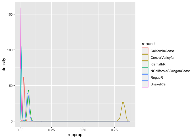
Following on from the above example, we will use
trace_subset to compute the equal-tail 95% credible
intervals for the 6 most abundant reporting units in the
rec1 fishery:
top6_cis <- trace_subset %>%
  group_by(repunit) %>%
  summarise(loCI = quantile(repprop, probs = 0.025),
            hiCI = quantile(repprop, probs = 0.975))
#> `summarise()` ungrouping output (override with `.groups` argument)

top6_cis
#> # A tibble: 6 x 3
#>   repunit                     loCI   hiCI
#>   <chr>                      <dbl>  <dbl>
#> 1 CaliforniaCoast         1.84e- 2 0.0443
#> 2 CentralValleyfa         7.88e- 1 0.847
#> 3 KlamathR                4.98e- 2 0.0875
#> 4 NCaliforniaSOregonCoast 2.99e- 3 0.0184
#> 5 RogueR                  4.37e- 2 0.0826
#> 6 SnakeRfa 2.56e-89 0.0119Sometimes totally unexpected things happen. One situation we saw in the California Chinook fishery was samples coming to us that were actually coho salmon. Before we included coho salmon in the reference sample, these coho always assigned quite strongly to Alaska populations of Chinook, even though they don’t really look like Chinook at all.
In this case, it is useful to look at the raw log-likelihood values
computed for the individual, rather than the scaled posterior
probabilities. Because aberrantly low values of the genotype
log-likelihood can indicate that there is something wrong. However, the
raw likelihood that you get will depend on the number of missing loci,
etc. rubias deals with this by computing a z-score
for each fish. The Z-score is the Z statistic obtained from the fish’s
log-likelihood (by subtracting from it the expected log-likelihood and
dividing by the expected standard deviation). rubias’s
implementation of the z-score accounts for the pattern of missing data,
but it does this without all the simulation that gsi_sim
does. This makes it much, much, faster—fast enough that we can compute
it be default for every fish and every population.
Here, we will look at the z-score computed for each fish to the population with the highest posterior. (It is worth noting that you would never want to use the z-score to assign fish to different populations—it is only there to decide whether it looks like it might not have actually come from the population that it was assigned to, or any other population in the reference data set.)
# get the maximum-a-posteriori population for each individual
map_rows <- mix_est$indiv_posteriors %>%
  group_by(indiv) %>%
  top_n(1, PofZ) %>%
  ungroup()
If everything is kosher, then we expect that the z-scores we see will be roughly normally distributed. We can compare the distribution of z-scores we see with a bunch of simulated normal random variables.
normo <- tibble(z_score = rnorm(1e06))
ggplot(map_rows, aes(x = z_score)) +
  geom_density(colour = "blue") +
  geom_density(data = normo, colour = "black")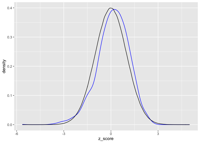
The normal density is in black and the distribution of our observed z_scores is in blue. They fit reasonably well, suggesting that there is not too much weird stuff going on overall. (That is good!)
The z_score statistic is most useful as a check for individuals. It is intended to be a quick way to identify aberrant individuals. If you see a z-score to the maximum-a-posteriori population for an individual in your mixture sample that is considerably less than z_scores you saw in the reference, then you might infer that the individual doesn’t actually fit any of the populations in the reference well.
Here I include a small, contrived example. We use the
small_chinook data set so that it goes fast.
First, we analyze the data with no fish in the mixture of known collection
no_kc <- infer_mixture(small_chinook_ref, small_chinook_mix, gen_start_col = 5)
#> Collating data; compiling reference allele frequencies, etc.   time: 0.20 seconds
#> Computing reference locus specific means and variances for computing mixture z-scores   time: 0.02 seconds
#> Working on mixture collection: rec3 with 29 individuals
#>   calculating log-likelihoods of the mixture individuals.   time: 0.01 seconds
#>   performing 2000 total sweeps, 100 of which are burn-in and will not be used in computing averages in method "MCMC"   time: 0.03 seconds
#>   tidying output into a tibble.   time: 0.03 seconds
#> Working on mixture collection: rec1 with 36 individuals
#>   calculating log-likelihoods of the mixture individuals.   time: 0.01 seconds
#>   performing 2000 total sweeps, 100 of which are burn-in and will not be used in computing averages in method "MCMC"   time: 0.03 seconds
#>   tidying output into a tibble.   time: 0.03 seconds
#> Working on mixture collection: rec2 with 35 individuals
#>   calculating log-likelihoods of the mixture individuals.   time: 0.01 seconds
#>   performing 2000 total sweeps, 100 of which are burn-in and will not be used in computing averages in method "MCMC"   time: 0.03 seconds
#>   tidying output into a tibble.   time: 0.03 seconds
And look at the results for the mixing proportions:
no_kc$mixing_proportions %>%
  arrange(mixture_collection, desc(pi))
#> # A tibble: 18 x 4
#>    mixture_collection repunit         collection          pi
#>    <chr>              <chr>           <chr>            <dbl>
#>  1 rec1               CentralValleyfa Feather_H_fa   0.849
#>  2 rec1               CentralValleysp Deer_Cr_sp     0.0508
#>  3 rec1               CaliforniaCoast Eel_R          0.0400
#>  4 rec1               KlamathR        Klamath_IGH_fa 0.0305
#>  5 rec1               MidOregonCoast  Umpqua_sp      0.0252
#>  6 rec1               CentralValleywi Sacramento_H   0.00463
#>  7 rec2               CentralValleyfa Feather_H_fa   0.809
#>  8 rec2               KlamathR        Klamath_IGH_fa 0.103
#>  9 rec2               MidOregonCoast  Umpqua_sp      0.0733
#> 10 rec2               CentralValleysp Deer_Cr_sp     0.00550
#> 11 rec2               CaliforniaCoast Eel_R          0.00479
#> 12 rec2               CentralValleywi Sacramento_H   0.00474
#> 13 rec3               CentralValleyfa Feather_H_fa   0.839
#> 14 rec3               CaliforniaCoast Eel_R          0.0714
#> 15 rec3               MidOregonCoast  Umpqua_sp      0.0496
#> 16 rec3               KlamathR        Klamath_IGH_fa 0.0262
#> 17 rec3               CentralValleysp Deer_Cr_sp     0.00875
#> 18 rec3               CentralValleywi Sacramento_H   0.00542
Now, we will do the same analysis, but pretend that we know that the first 8 of the 36 fish in fishery rec1 are from the Deer_Cr_sp collection.
First we have to add the known_collection column to the reference.
# make reference file that includes the known_collection column
kc_ref <- small_chinook_ref %>%
  mutate(known_collection = collection) %>%
  select(known_collection, everything())

# see what that looks like
kc_ref[1:10, 1:8]
#> # A tibble: 10 x 8
#>    known_collection sample_type repunit collection indiv Ots_94857.232
#>    <chr>            <chr>       <chr>   <chr>      <chr>         <int>
#>  1 Deer_Cr_sp       reference   Centra… Deer_Cr_sp Deer…             2
#>  2 Deer_Cr_sp       reference   Centra… Deer_Cr_sp Deer…             2
#>  3 Deer_Cr_sp       reference   Centra… Deer_Cr_sp Deer…             2
#>  4 Deer_Cr_sp       reference   Centra… Deer_Cr_sp Deer…             4
#>  5 Deer_Cr_sp       reference   Centra… Deer_Cr_sp Deer…             2
#>  6 Deer_Cr_sp       reference   Centra… Deer_Cr_sp Deer…             4
#>  7 Deer_Cr_sp       reference   Centra… Deer_Cr_sp Deer…             2
#>  8 Deer_Cr_sp       reference   Centra… Deer_Cr_sp Deer…             4
#>  9 Deer_Cr_sp       reference   Centra… Deer_Cr_sp Deer…             2
#> 10 Deer_Cr_sp       reference   Centra… Deer_Cr_sp Deer…             2
#> # … with 2 more variables: Ots_94857.232.1 <int>, Ots_102213.210 <int>
Then we add the known collection column to the mixture. We start out making it all NAs, and then we change that to Deer_Cr_sp for 8 of the rec1 fish:
kc_mix <- small_chinook_mix %>%
  mutate(known_collection = NA) %>%
  select(known_collection, everything())

kc_mix$known_collection[kc_mix$collection == "rec1"][1:8] <- "Deer_Cr_sp"

# here is what that looks like now (dropping most of the genetic data columns)
kc_mix[1:20, 1:7]
#> # A tibble: 20 x 7
#>    known_collection sample_type repunit collection indiv Ots_94857.232
#>    <chr>            <chr>       <chr>   <chr>      <chr>         <int>
#>  1 <NA>             mixture     <NA>    rec3       T125…             4
#>  2 Deer_Cr_sp       mixture     <NA>    rec1       T127…             4
#>  3 <NA>             mixture     <NA>    rec2       T124…             4
#>  4 <NA>             mixture     <NA>    rec2       T127…             2
#>  5 <NA>             mixture     <NA>    rec3       T127…             4
#>  6 Deer_Cr_sp       mixture     <NA>    rec1       T127…             4
#>  7 <NA>             mixture     <NA>    rec3       T124…             4
#>  8 Deer_Cr_sp       mixture     <NA>    rec1       T126…             2
#>  9 <NA>             mixture     <NA>    rec3       T125…             4
#> 10 Deer_Cr_sp       mixture     <NA>    rec1       T127…             4
#> 11 Deer_Cr_sp       mixture     <NA>    rec1       T127…             2
#> 12 Deer_Cr_sp       mixture     <NA>    rec1       T127…             2
#> 13 <NA>             mixture     <NA>    rec2       T126…             4
#> 14 <NA>             mixture     <NA>    rec3       T126…             4
#> 15 <NA>             mixture     <NA>    rec2       T125…             4
#> 16 Deer_Cr_sp       mixture     <NA>    rec1       T126…             4
#> 17 <NA>             mixture     <NA>    rec2       T124…             4
#> 18 <NA>             mixture     <NA>    rec3       T124…             2
#> 19 Deer_Cr_sp       mixture     <NA>    rec1       T124…             4
#> 20 <NA>             mixture     <NA>    rec3       T125…             2
#> # … with 1 more variable: Ots_94857.232.1 <int>
And now we can do the mixture analysis:
# note that the genetic data start in column 6 now
with_kc <- infer_mixture(kc_ref, kc_mix, 6)
#> Collating data; compiling reference allele frequencies, etc.   time: 0.20 seconds
#> Computing reference locus specific means and variances for computing mixture z-scores   time: 0.02 seconds
#> Working on mixture collection: rec3 with 29 individuals
#>   calculating log-likelihoods of the mixture individuals.   time: 0.01 seconds
#>   performing 2000 total sweeps, 100 of which are burn-in and will not be used in computing averages in method "MCMC"   time: 0.03 seconds
#>   tidying output into a tibble.   time: 0.03 seconds
#> Working on mixture collection: rec1 with 36 individuals
#>   calculating log-likelihoods of the mixture individuals.   time: 0.01 seconds
#>   performing 2000 total sweeps, 100 of which are burn-in and will not be used in computing averages in method "MCMC"   time: 0.03 seconds
#>   tidying output into a tibble.   time: 0.03 seconds
#> Working on mixture collection: rec2 with 35 individuals
#>   calculating log-likelihoods of the mixture individuals.   time: 0.01 seconds
#>   performing 2000 total sweeps, 100 of which are burn-in and will not be used in computing averages in method "MCMC"   time: 0.03 seconds
#>   tidying output into a tibble.   time: 0.03 seconds
And, when we look at the estimated proportions, we see that for rec1 they reflect the fact that 8 of those fish were singled out as known fish from Deer_Ck_sp:
with_kc$mixing_proportions %>%
  arrange(mixture_collection, desc(pi))
#> # A tibble: 18 x 4
#>    mixture_collection repunit         collection          pi
#>    <chr>              <chr>           <chr>            <dbl>
#>  1 rec1               CentralValleyfa Feather_H_fa   0.546
#>  2 rec1               CentralValleysp Deer_Cr_sp     0.355
#>  3 rec1               CaliforniaCoast Eel_R          0.0411
#>  4 rec1               KlamathR        Klamath_IGH_fa 0.0318
#>  5 rec1               MidOregonCoast  Umpqua_sp      0.0220
#>  6 rec1               CentralValleywi Sacramento_H   0.00438
#>  7 rec2               CentralValleyfa Feather_H_fa   0.806
#>  8 rec2               KlamathR        Klamath_IGH_fa 0.104
#>  9 rec2               MidOregonCoast  Umpqua_sp      0.0732
#> 10 rec2               CentralValleysp Deer_Cr_sp     0.00688
#> 11 rec2               CaliforniaCoast Eel_R          0.00551
#> 12 rec2               CentralValleywi Sacramento_H   0.00456
#> 13 rec3               CentralValleyfa Feather_H_fa   0.835
#> 14 rec3               CaliforniaCoast Eel_R          0.0732
#> 15 rec3               MidOregonCoast  Umpqua_sp      0.0494
#> 16 rec3               KlamathR        Klamath_IGH_fa 0.0281
#> 17 rec3               CentralValleysp Deer_Cr_sp     0.00883
#> 18 rec3               CentralValleywi Sacramento_H   0.00565
The output from infer_mixture() in this case can be used
just like it was before without known individuals in the baseline.
The default model in rubias is a conditional model in
which inference is done with the baseline allele counts fixed. In a
fully Bayesian version, fish from within the mixture that are allocated
(on any particular step of the MCMC) to one of the reference samples
have their alleles added to that reference sample, thus (one hopes)
refining the estimate of allele frequencies in that sample. This is more
computationally intensive, and, is done using parallel computation, by
default running one thread for every core on your machine.
The basic way to invoke the fully Bayesian model is to use the
infer_mixture function with the method option
set to “BR”. For example:
full_model_results <- infer_mixture(
  reference = chinook,
  mixture = chinook_mix,
  gen_start_col = 5,
  method = "BR"
  )
More details about different options for working with the fully Bayesian model are available in the vignette about the fully Bayesian model.
A standard analysis in molecular ecology is to assign individuals in
the reference back to the collections in the reference using a
leave-one-out procedure. This is taken care of by the
self_assign() function.
sa_chinook <- self_assign(reference = chinook, gen_start_col = 5)
#> Summary Statistics:
#>
#> 7301 Individuals in Sample
#>
#> 91 Loci: AldB1.122, AldoB4.183, OTNAML12_1.SNP1, Ots_100884.287, Ots_101119.381, Ots_101704.143, Ots_102213.210, Ots_102414.395, Ots_102420.494, Ots_102457.132, Ots_102801.308, Ots_102867.609, Ots_103041.52, Ots_104063.132, Ots_104569.86, Ots_105105.613, Ots_105132.200, Ots_105401.325, Ots_105407.117, Ots_106499.70, Ots_106747.239, Ots_107074.284, Ots_107285.93, Ots_107806.821, Ots_108007.208, Ots_108390.329, Ots_108735.302, Ots_109693.392, Ots_110064.383, Ots_110201.363, Ots_110495.380, Ots_110551.64, Ots_111312.435, Ots_111666.408, Ots_111681.657, Ots_112301.43, Ots_112419.131, Ots_112820.284, Ots_112876.371, Ots_113242.216, Ots_113457.40, Ots_117043.255, Ots_117242.136, Ots_117432.409, Ots_118175.479, Ots_118205.61, Ots_118938.325, Ots_122414.56, Ots_123048.521, Ots_123921.111, Ots_124774.477, Ots_127236.62, Ots_128302.57, Ots_128693.461, Ots_128757.61, Ots_129144.472, Ots_129170.683, Ots_129458.451, Ots_130720.99, Ots_131460.584, Ots_131906.141, Ots_94857.232, Ots_96222.525, Ots_96500.180, Ots_97077.179, Ots_99550.204, Ots_ARNT.195, Ots_AsnRS.60, Ots_aspat.196, Ots_CD59.2, Ots_CD63, Ots_EP.529, Ots_GDH.81x, Ots_HSP90B.385, Ots_MHC1, Ots_mybp.85, Ots_myoD.364, Ots_Ots311.101x, Ots_PGK.54, Ots_Prl2, Ots_RFC2.558, Ots_SClkF2R2.135, Ots_SWS1op.182, Ots_TAPBP, Ots_u07.07.161, Ots_u07.49.290, Ots_u4.92, OTSBMP.2.SNP1, OTSTF1.SNP1, S71.336, unk_526
#>
#> 39 Reporting Units: CentralValleyfa, CentralValleysp, CentralValleywi, CaliforniaCoast, KlamathR, NCaliforniaSOregonCoast, RogueR, MidOregonCoast, NOregonCoast, WillametteR, DeschutesRfa, LColumbiaRfa, LColumbiaRsp, MidColumbiaRtule, UColumbiaRsufa, MidandUpperColumbiaRsp, SnakeRfa, SnakeRspsu, NPugetSound, WashingtonCoast, SPugetSound, LFraserR, LThompsonR, EVancouverIs, WVancouverIs, MSkeenaR, MidSkeenaR, LSkeenaR, SSEAlaska, NGulfCoastAlsekR, NGulfCoastKarlukR, TakuR, NSEAlaskaChilkatR, NGulfCoastSitukR, CopperR, SusitnaR, LKuskokwimBristolBay, MidYukon, CohoSp
#>
#> 69 Collections: Feather_H_sp, Butte_Cr_Sp, Mill_Cr_sp, Deer_Cr_sp, UpperSacramento_R_sp, Feather_H_fa, Butte_Cr_fa, Mill_Cr_fa, Deer_Cr_fa, Mokelumne_R_fa, Battle_Cr, Sacramento_R_lf, Sacramento_H, Eel_R, Russian_R, Klamath_IGH_fa, Trinity_H_sp, Smith_R, Chetco_R, Cole_Rivers_H, Applegate_Cr, Coquille_R, Umpqua_sp, Nestucca_H, Siuslaw_R, Alsea_R, Nehalem_R, Siletz_R, N_Santiam_H, McKenzie_H, L_Deschutes_R, Cowlitz_H_fa, Cowlitz_H_sp, Kalama_H_sp, Spring_Cr_H, Hanford_Reach, PriestRapids_H, Wells_H, Wenatchee_R, CleElum, Lyons_Ferry_H, Rapid_R_H, McCall_H, Kendall_H_sp, Forks_Cr_H, Soos_H, Marblemount_H_sp, QuinaltLake_f, Harris_R, Birkenhead_H, Spius_H, Big_Qual_H, Robertson_H, Morice_R, Kitwanga_R, L_Kalum_R, LPW_Unuk_R, Goat_Cr, Karluk_R, LittleTatsamenie, Tahini_R, Situk_R, Sinona_Ck, Montana_Ck, George_R, Kanektok_R, Togiak_R, Kantishna_R, California_Coho
#>
#> 4.18% of allelic data identified as missing
Now, you can look at the self assignment results:
head(sa_chinook, n = 100)
#> # A tibble: 100 x 11
#>    indiv collection repunit inferred_collec… inferred_repunit scaled_likeliho…
#>    <chr> <chr>      <chr>   <chr>            <chr>                       <dbl>
#>  1 Feat… Feather_H… Centra… Feather_H_sp     CentralValleyfa           0.629
#>  2 Feat… Feather_H… Centra… Feather_H_fa     CentralValleyfa           0.161
#>  3 Feat… Feather_H… Centra… Butte_Cr_fa      CentralValleyfa           0.0612
#>  4 Feat… Feather_H… Centra… Mill_Cr_sp       CentralValleysp           0.0400
#>  5 Feat… Feather_H… Centra… Mill_Cr_fa       CentralValleyfa           0.0288
#>  6 Feat… Feather_H… Centra… UpperSacramento… CentralValleysp           0.0285
#>  7 Feat… Feather_H… Centra… Deer_Cr_sp       CentralValleysp           0.0236
#>  8 Feat… Feather_H… Centra… Butte_Cr_Sp      CentralValleysp           0.00852
#>  9 Feat… Feather_H… Centra… Battle_Cr        CentralValleyfa           0.00779
#> 10 Feat… Feather_H… Centra… Mokelumne_R_fa   CentralValleyfa           0.00592
#> # … with 90 more rows, and 5 more variables: log_likelihood <dbl>,
#> #   z_score <dbl>, n_non_miss_loci <int>, n_miss_loci <int>,
#> #   missing_loci <list>
The log_likelihood is the log probability of the fish’s
genotype given it is from the inferred_collection computed
using leave-one-out. The scaled_likelihood is the posterior
prob of assigning the fish to the inferred_collection given
an equal prior on every collection in the reference. Other columns are
as in the output for infer_mixture(). Note that the
z_score computed here can be used to assess the
distribution of the z_score statistic for fish from known,
reference populations. This can be used to compare to values obtained in
mixed fisheries.
The output can be summarized by repunit as was done above:
sa_to_repu <- sa_chinook %>%
  group_by(indiv, collection, repunit, inferred_repunit) %>%
  summarise(repu_scaled_like = sum(scaled_likelihood))
#> `summarise()` regrouping output by 'indiv', 'collection', 'repunit' (override with `.groups` argument)

head(sa_to_repu, n = 200)
#> # A tibble: 200 x 5
#> # Groups:   indiv, collection, repunit [6]
#>    indiv        collection repunit      inferred_repunit repu_scaled_like
#>    <chr>        <chr>      <chr>        <chr>                       <dbl>
#>  1 Alsea_R:0001 Alsea_R    NOregonCoast CaliforniaCoast          3.72e- 8
#>  2 Alsea_R:0001 Alsea_R    NOregonCoast CentralValleyfa          1.54e-14
#>  3 Alsea_R:0001 Alsea_R    NOregonCoast CentralValleysp          8.12e-15
#>  4 Alsea_R:0001 Alsea_R    NOregonCoast CentralValleywi          1.22e-23
#>  5 Alsea_R:0001 Alsea_R    NOregonCoast CohoSp                   2.09e-52
#>  6 Alsea_R:0001 Alsea_R    NOregonCoast CopperR                  3.08e-20
#>  7 Alsea_R:0001 Alsea_R    NOregonCoast DeschutesRfa             3.81e-10
#>  8 Alsea_R:0001 Alsea_R    NOregonCoast EVancouverIs             1.02e- 8
#>  9 Alsea_R:0001 Alsea_R    NOregonCoast KlamathR                 1.11e-11
#> 10 Alsea_R:0001 Alsea_R    NOregonCoast LColumbiaRfa             8.52e- 8
#> # … with 190 more rowsIf you want to know how much accuracy you can expect given a set of
genetic markers and a grouping of populations (collections)
into reporting units (repunits), there are two different
functions you might use:
assess_reference_loo(): This function carries out
simulation of mixtures using the leave-one-out approach of Anderson,
Waples, and Kalinowski (2008).assess_reference_mc(): This functions breaks the
reference data set into different subsets, one of which is used as the
reference data set and the other the mixture. It is difficult to
simulate very large mixture samples using this method, because it is
constrained by the number of fish in the reference data set.Both of the functions take two required arguments: 1) a data frame of reference genetic data, and 2) the number of the column in which the genetic data start.
Here we use the chinook data to simulate 50 mixture
samples of size 200 fish using the default values (Dirichlet parameters
of 1.5 for each reporting unit, and Dirichlet parameters of 1.5 for each
collection within a reporting unit…)
chin_sims <- assess_reference_loo(reference = chinook,
                     gen_start_col = 5,
                     reps = 50,
                     mixsize = 200)
Here is what the output looks like:
chin_sims
#> # A tibble: 3,450 x 9
#>    repunit_scenario collection_scen…  iter repunit collection true_pi     n
#>    <chr>            <chr>            <int> <chr>   <chr>        <dbl> <dbl>
#>  1 1                1                    1 Centra… Feather_H… 8.42e-4     0
#>  2 1                1                    1 Centra… Butte_Cr_… 6.55e-4     0
#>  3 1                1                    1 Centra… Mill_Cr_sp 1.37e-3     0
#>  4 1                1                    1 Centra… Deer_Cr_sp 4.41e-3     1
#>  5 1                1                    1 Centra… UpperSacr… 6.25e-4     0
#>  6 1                1                    1 Centra… Feather_H… 2.89e-3     2
#>  7 1                1                    1 Centra… Butte_Cr_… 8.50e-4     0
#>  8 1                1                    1 Centra… Mill_Cr_fa 2.86e-3     1
#>  9 1                1                    1 Centra… Deer_Cr_fa 6.53e-3     0
#> 10 1                1                    1 Centra… Mokelumne… 8.99e-4     0
#> # … with 3,440 more rows, and 2 more variables: post_mean_pi <dbl>,
#> #   mle_pi <dbl>
The columns here are:
repunit_scenario and integer that gives that repunit
simulation parameters (see below about simulating multiple
scenarios).collections_scenario and integer that gives that
collection simulation paramters (see below about simulating multiple
scenarios).iter the simulation number (1 up to
reps)repunit the reporting unitcollection the collectiontrue_pi the true simulated mixing proportionn the actual number of fish from the collection in the
simulated mixture.post_mean_pi the posterior mean of mixing
proportion.mle_pi the maximum likelihood of pi
obtained using an EM-algorithm.assess_reference_loo()By default, each iteration, the proportions of fish from each reporting unit are simulated from a Dirichlet distribution with parameter (1.5,…,1.5). And, within each reporting unit the mixing proportions from different collections are drawn from a Dirichlet distribution with parameter (1.5,…,1.5).
The value of 1.5 for the Dirichlet parameter for reporting units can
be changed using the alpha_repunit. The Dirichlet parameter
for collections can be set using the alpha_collection
parameter.
Sometimes, however, more control over the composition of the
simulated mixtures is desired. This is achieved by passing a two-column
data.frame to either alpha_repunit or
alpha_collection (or both). If you are passing the
data.frame in for alpha_repunit, the first column must be
named repunit and it must contain a character vector
specifying reporting units. In the data.frame for
alpha_collection the first column must be named
collection and must hold a character vector specifying
different collections. It is an error if a repunit or collection is
specified that does not exist in the reference. However, you do not need
to specify a value for every reporting unit or collection. (If they are
absent, the value is assumed to be zero.)
The second column of the data frame must be one of
count, ppn or dirichlet. These
specify, respectively,
ppn values will be normalized to sum to one if they
do not. As such, they can be regarded as weights.Let’s say that we want to simulate data that roughly have proportions
like what we saw in the Chinook rec1 fishery. We have those
estimates in the variable top6:
top6
#> # A tibble: 6 x 3
#> # Groups:   mixture_collection [1]
#>   mixture_collection repunit                 repprop
#>   <chr>              <chr>                     <dbl>
#> 1 rec1               CentralValleyfa         0.819
#> 2 rec1               KlamathR                0.0675
#> 3 rec1               RogueR                  0.0608
#> 4 rec1               CaliforniaCoast         0.0298
#> 5 rec1               NCaliforniaSOregonCoast 0.00927
#> 6 rec1               SnakeRfa                0.00320
We could, if we put those repprop values into a
ppn column, simulate mixtures with exactly those
proportions. Or if we wanted to simulate exact numbers of fish in a
sample of 346 fish, we could get those values like this:
round(top6$repprop * 350)
#> [1] 287  24  21  10   3   1
and then put them in a cnts column.
However, in this case, we want to simulate mixtures that look similar
to the one we estimated, but have some variation. For that we will want
to supply Dirichlet random variable paramaters in a column named
dirichlet. If we make the values proportional to the mixing
proportions, then, on average that is what they will be. If the values
are large, then there will be little variation between simulated
mixtures. And if the the values are small there will be lots of
variation. We’ll scale them so that they sum to 10—that should give some
variation, but not too much. Accordingly the tibble that we pass in as
the alpha_repunit parameter, which describes the variation
in reporting unit proportions we would like to simulate would look like
this:
arep <- top6 %>%
  ungroup() %>%
  mutate(dirichlet = 10 * repprop) %>%
  select(repunit, dirichlet)

arep
#> # A tibble: 6 x 2
#>   repunit                 dirichlet
#>   <chr>                       <dbl>
#> 1 CentralValleyfa            8.19
#> 2 KlamathR                   0.675
#> 3 RogueR                     0.608
#> 4 CaliforniaCoast            0.298
#> 5 NCaliforniaSOregonCoast    0.0927
#> 6 SnakeRfa                   0.0320
Let’s do some simulations with those repunit parameters. By default, if we don’t specify anything extra for the collections, they get dirichlet parameters of 1.5.
chin_sims_repu_top6 <- assess_reference_loo(reference = chinook,
                     gen_start_col = 5,
                     reps = 50,
                     mixsize = 200,
                     alpha_repunit = arep)
Now, we can summarise the output by reporting unit…
# now, call those repunits that we did not specify in arep "OTHER"
# and then sum up over reporting units
tmp <- chin_sims_repu_top6 %>%
  mutate(repunit = ifelse(repunit %in% arep$repunit, repunit, "OTHER")) %>%
  group_by(iter, repunit) %>%
  summarise(true_repprop = sum(true_pi),
            reprop_posterior_mean = sum(post_mean_pi),
            repu_n = sum(n)) %>%
  mutate(repu_n_prop = repu_n / sum(repu_n))
#> `summarise()` regrouping output by 'iter' (override with `.groups` argument)
…and then plot it for the values we are interested in:
# then plot them
ggplot(tmp, aes(x = true_repprop, y = reprop_posterior_mean, colour = repunit)) +
  geom_point() +
  geom_abline(intercept = 0, slope = 1) +
  facet_wrap(~ repunit)
Or plot comparing to their “n” value, which is the actual number of fish from each reporting unit in the sample.
ggplot(tmp, aes(x = repu_n_prop, y = reprop_posterior_mean, colour = repunit)) +
  geom_point() +
  geom_abline(intercept = 0, slope = 1) +
  facet_wrap(~ repunit)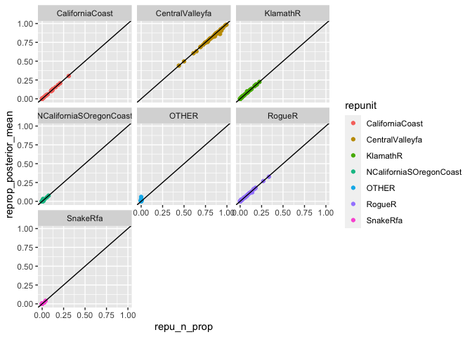
Quite often you might be curious about how much you can expect to be
able to trust the posterior for individual fish from a mixture like
this. You can retrieve all the posteriors computed for the fish
simulated in assess_reference_loo() using the
return_indiv_posteriors option. When you do this, the
function returns a list with components mixture_proportions
(which holds a tibble like chin_sims_repu_top6 in the
previous section) and indiv_posteriors, which holds all the
posteriors (PofZs) for the simulated individuals.
set.seed(100)
chin_sims_with_indivs <- assess_reference_loo(reference = chinook,
                     gen_start_col = 5,
                     reps = 50,
                     mixsize = 200,
                     alpha_repunit = arep,
                     return_indiv_posteriors = TRUE)
#> Warning: `as.tibble()` is deprecated as of tibble 2.0.0.
#> Please use `as_tibble()` instead.
#> The signature and semantics have changed, see `?as_tibble`.
#> This warning is displayed once every 8 hours.
#> Call `lifecycle::last_warnings()` to see where this warning was generated.

# print out the indiv posteriors
chin_sims_with_indivs$indiv_posteriors
#> # A tibble: 690,000 x 9
#>    repunit_scenario collection_scen…  iter indiv simulated_repun…
#>    <chr>            <chr>            <int> <int> <chr>
#>  1 1                1                    1     1 CentralValleyfa
#>  2 1                1                    1     1 CentralValleyfa
#>  3 1                1                    1     1 CentralValleyfa
#>  4 1                1                    1     1 CentralValleyfa
#>  5 1                1                    1     1 CentralValleyfa
#>  6 1                1                    1     1 CentralValleyfa
#>  7 1                1                    1     1 CentralValleyfa
#>  8 1                1                    1     1 CentralValleyfa
#>  9 1                1                    1     1 CentralValleyfa
#> 10 1                1                    1     1 CentralValleyfa
#> # … with 689,990 more rows, and 4 more variables: simulated_collection <chr>,
#> #   repunit <chr>, collection <chr>, PofZ <dbl>
In this tibble: - indiv is an integer specifier of the
simulated individual - simulated_repunit is the reporting
unit the individual was simulated from -
simulated_collection is the collection the simulated
genotype came from - PofZ is the mean over the MCMC of the
posterior probability that the individual originated from the
collection.
Now that we have done that, we can see what the distribution of posteriors to the correct reporting unit is for fish from the different simulated collections. We’ll do that with a boxplot, coloring by repunit:
# summarise things
repu_pofzs <- chin_sims_with_indivs$indiv_posteriors %>%
  filter(repunit == simulated_repunit) %>%
  group_by(iter, indiv, simulated_collection, repunit) %>%  # first aggregate over reporting units
  summarise(repu_PofZ = sum(PofZ)) %>%
  ungroup() %>%
  arrange(repunit, simulated_collection) %>%
  mutate(simulated_collection = factor(simulated_collection, levels = unique(simulated_collection)))
#> `summarise()` regrouping output by 'iter', 'indiv', 'simulated_collection' (override with `.groups` argument)

# also get the number of simulated individuals from each collection
num_simmed <- chin_sims_with_indivs$indiv_posteriors %>%
  group_by(iter, indiv) %>%
  slice(1) %>%
  ungroup() %>%
  count(simulated_collection)

# note, the last few steps make simulated collection a factor so that collections within
# the same repunit are grouped together in the plot.

# now, plot it
ggplot(repu_pofzs, aes(x = simulated_collection, y = repu_PofZ)) +
  geom_boxplot(aes(colour = repunit)) +
  geom_text(data = num_simmed, mapping = aes(y = 1.025, label = n), angle = 90, hjust = 0, vjust = 0.5, size = 3) +
  theme(axis.text.x = element_text(angle = 90, hjust = 1, size = 9, vjust = 0.5)) +
  ylim(c(NA, 1.05))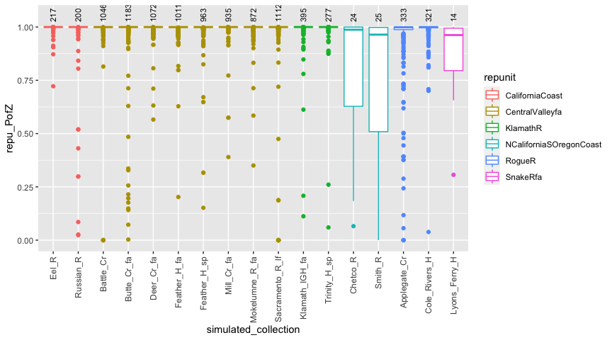
Great. That is helpful.
By default, individuals are simulated in
assess_reference_loo() by resampling full multilocus
genotypes. This tends to be more realistic, because it includes as
missing in the simulations all the missing data for individuals in the
reference. However, as all the genes in individuals that have been
incorrectly placed in a reference stay together, that individual might
have a low value of PofZ to the population it was simulated from. Due to
the latter issue, it might also yield a more pessimistic assessment’ of
the power for GSI.
An alternative is to resample over gene copies—the CV-GC method of Anderson, Waples, and Kalinowski (2008).
Let us do that and see how the simulated PofZ results change. Here we do the simulations…
set.seed(101) # for reproducibility
# do the simulation
chin_sims_by_gc <- assess_reference_loo(reference = chinook,
                     gen_start_col = 5,
                     reps = 50,
                     mixsize = 200,
                     alpha_repunit = arep,
                     return_indiv_posteriors = TRUE,
                     resampling_unit = "gene_copies")
and here we process the output and plot it:
# summarise things
repu_pofzs_gc <- chin_sims_by_gc$indiv_posteriors %>%
  filter(repunit == simulated_repunit) %>%
  group_by(iter, indiv, simulated_collection, repunit) %>%  # first aggregate over reporting units
  summarise(repu_PofZ = sum(PofZ)) %>%
  ungroup() %>%
  arrange(repunit, simulated_collection) %>%
  mutate(simulated_collection = factor(simulated_collection, levels = unique(simulated_collection)))
#> `summarise()` regrouping output by 'iter', 'indiv', 'simulated_collection' (override with `.groups` argument)

# also get the number of simulated individuals from each collection
num_simmed_gc <- chin_sims_by_gc$indiv_posteriors %>%
  group_by(iter, indiv) %>%
  slice(1) %>%
  ungroup() %>%
  count(simulated_collection)

# note, the last few steps make simulated collection a factor so that collections within
# the same repunit are grouped together in the plot.

# now, plot it
ggplot(repu_pofzs_gc, aes(x = simulated_collection, y = repu_PofZ)) +
  geom_boxplot(aes(colour = repunit)) +
  geom_text(data = num_simmed_gc, mapping = aes(y = 1.025, label = n), angle = 90, hjust = 0, vjust = 0.5, size = 3) +
  theme(axis.text.x = element_text(angle = 90, hjust = 1, size = 9, vjust = 0.5)) +
  ylim(c(NA, 1.05))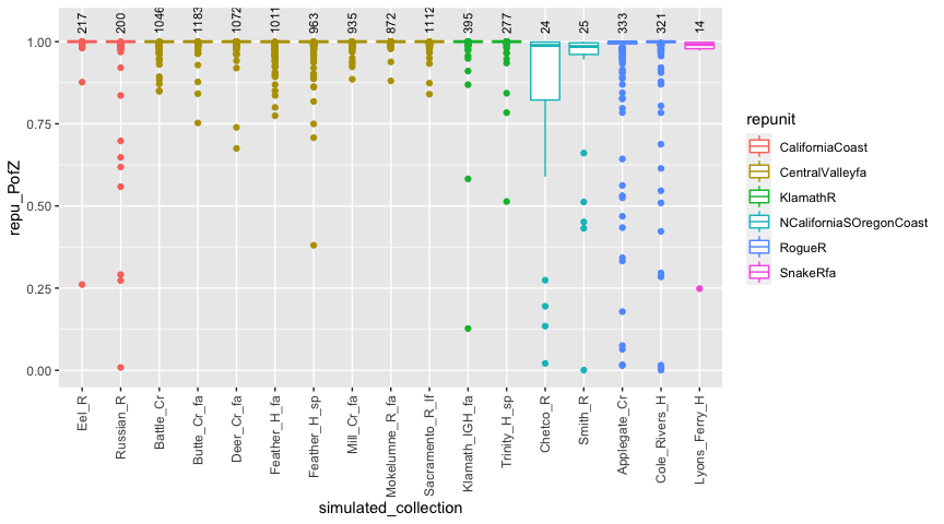
And in that, we find somewhat fewer fish that have low posteriors, but there are still some. This reminds us that with this dataset, (rather) occasionally it is possible to get individuals carrying genotypes that make it difficult to correctly assign them to reporting unit.
If you are simulating the reporting unit proportions or numbers, and
want to have more control over which collections those fish are
simulated from, within the reporting units, then the
sub_ppn and sub_dirichlet settings are for
you. These are given as column names in the
alpha_collection data frame.
For example, let’s say we want to simulate reporting unit proportions
as before, using arep from above:
arep
#> # A tibble: 6 x 2
#>   repunit                 dirichlet
#>   <chr>                       <dbl>
#> 1 CentralValleyfa            8.19
#> 2 KlamathR                   0.675
#> 3 RogueR                     0.608
#> 4 CaliforniaCoast            0.298
#> 5 NCaliforniaSOregonCoast    0.0927
#> 6 SnakeRfa                   0.0320
But, now, let’s say that within reporting unit we want specific weights for different collections. Then we could specify those, for example, like this:
arep_subs <- tribble(
  ~collection, ~sub_ppn,
  "Eel_R",   0.1,
  "Russian_R", 0.9,
  "Butte_Cr_fa", 0.7,
  "Feather_H_sp", 0.3
)
Collections that are not listed are given equal proportions within repunits that had no collections listed. However, if a collection is not listed, but other collections within its repunit are, then its simulated proportion will be zero. (Technically, it is not zero, but it is so small—like (10^{-8}) that is is effectively 0…doing that made coding it up a lot easier…)
Now, we can simulate with that and see what the resulting proportion of fish from each collection is:
chin_sims_sub_ppn <- assess_reference_loo(reference = chinook,
                     gen_start_col = 5,
                     reps = 50,
                     mixsize = 200,
                     alpha_repunit = arep,
                     alpha_collection = arep_subs,
                     return_indiv_posteriors = FALSE)  # don't bother returning individual posteriors
Now observe the average proportions of the collections and repunits that were simulated, and the average fraction, within reporting units of each of the collection
chin_sims_sub_ppn %>%
  group_by(repunit, collection) %>%
  summarise(mean_pi = mean(true_pi)) %>%
  group_by(repunit) %>%
  mutate(repunit_mean_pi = sum(mean_pi),
         fract_within = mean_pi / repunit_mean_pi) %>%
  mutate(fract_within = ifelse(fract_within < 1e-06, 0, fract_within))  %>% # anything less than 1 in a million gets called 0
  filter(repunit_mean_pi > 0.0)
#> `summarise()` regrouping output by 'repunit' (override with `.groups` argument)
#> # A tibble: 17 x 5
#> # Groups:   repunit [6]
#>    repunit               collection         mean_pi repunit_mean_pi fract_within
#>    <chr>                 <chr>                <dbl>           <dbl>        <dbl>
#>  1 CaliforniaCoast       Eel_R              3.57e-3         0.0357         0.1
#>  2 CaliforniaCoast       Russian_R          3.21e-2         0.0357         0.9
#>  3 CentralValleyfa       Battle_Cr          8.28e-8         0.828          0
#>  4 CentralValleyfa       Butte_Cr_fa        5.79e-1         0.828          0.700
#>  5 CentralValleyfa       Deer_Cr_fa         8.28e-8         0.828          0
#>  6 CentralValleyfa       Feather_H_fa       8.28e-8         0.828          0
#>  7 CentralValleyfa       Feather_H_sp       2.48e-1         0.828          0.300
#>  8 CentralValleyfa       Mill_Cr_fa         8.28e-8         0.828          0
#>  9 CentralValleyfa       Mokelumne_R_fa     8.28e-8         0.828          0
#> 10 CentralValleyfa       Sacramento_R_…     8.28e-8         0.828          0
#> 11 KlamathR              Klamath_IGH_fa     3.11e-2         0.0622         0.5
#> 12 KlamathR              Trinity_H_sp       3.11e-2         0.0622         0.5
#> 13 NCaliforniaSOregonCo… Chetco_R           5.51e-3         0.0110         0.5
#> 14 NCaliforniaSOregonCo… Smith_R            5.51e-3         0.0110         0.5
#> 15 RogueR                Applegate_Cr       2.69e-2         0.0539         0.5
#> 16 RogueR                Cole_Rivers_H      2.69e-2         0.0539         0.5
#> 17 SnakeRfa Lyons_Ferry_H 9.61e-3 0.00961 1In the fisheries world, “100% simulations” have been a staple. In
these simulations, mixtures are simulated in which 100% of the
individuals are from one collection (or reporting unit, I suppose). Eric
has never been a big fan of these since they don’t necessarily tell you
how you might do inferring actual mixtures that you might encounter.
Nonetheless, since they have been such a mainstay in the field, it is
worthwile showing how to do 100% simulations using rubias.
Furthermore, when people asked for this feature it made it clear that
Eric had to provide a way to simulate multiple different scenarios
without re-processing the reference data set each time. So this is what
I came up with: the way we do it is to pass a list of scenarios
to the alpha_repunit or alpha_collection
option in assess_reference_loo(). These can be named lists,
if desired. So, for example, let’s do 100% simulations for each of the
repunits in arep:
arep$repunit
#> [1] "CentralValleyfa"         "KlamathR"
#> [3] "RogueR"                  "CaliforniaCoast"
#> [5] "NCaliforniaSOregonCoast" "SnakeRfa"
We will let the collections within them just be drawn from a dirichlet distribution with parameter 10 (so, pretty close to equal proportions).
So, to do this, we make a list of data frames with the proportions. We’ll give it some names too:
six_hundy_scenarios <- lapply(arep$repunit, function(x) tibble(repunit = x, ppn = 1.0))
names(six_hundy_scenarios) <- paste("All", arep$repunit, sep = "-")
Then, we use it, producing only 5 replicates for each scenario:
repu_hundy_results <- assess_reference_loo(reference = chinook,
                     gen_start_col = 5,
                     reps = 5,
                     mixsize = 50,
                     alpha_repunit = six_hundy_scenarios,
                     alpha_collection = 10)
#> ++++ Starting in on repunit_scenario All-CentralValleyfa with collection scenario 1 ++++
#> Doing LOO simulations rep 1 of 5
#> Doing LOO simulations rep 2 of 5
#> Doing LOO simulations rep 3 of 5
#> Doing LOO simulations rep 4 of 5
#> Doing LOO simulations rep 5 of 5
#> ++++ Starting in on repunit_scenario All-KlamathR with collection scenario 1 ++++
#> Doing LOO simulations rep 1 of 5
#> Doing LOO simulations rep 2 of 5
#> Doing LOO simulations rep 3 of 5
#> Doing LOO simulations rep 4 of 5
#> Doing LOO simulations rep 5 of 5
#> ++++ Starting in on repunit_scenario All-RogueR with collection scenario 1 ++++
#> Doing LOO simulations rep 1 of 5
#> Doing LOO simulations rep 2 of 5
#> Doing LOO simulations rep 3 of 5
#> Doing LOO simulations rep 4 of 5
#> Doing LOO simulations rep 5 of 5
#> ++++ Starting in on repunit_scenario All-CaliforniaCoast with collection scenario 1 ++++
#> Doing LOO simulations rep 1 of 5
#> Doing LOO simulations rep 2 of 5
#> Doing LOO simulations rep 3 of 5
#> Doing LOO simulations rep 4 of 5
#> Doing LOO simulations rep 5 of 5
#> ++++ Starting in on repunit_scenario All-NCaliforniaSOregonCoast with collection scenario 1 ++++
#> Doing LOO simulations rep 1 of 5
#> Doing LOO simulations rep 2 of 5
#> Doing LOO simulations rep 3 of 5
#> Doing LOO simulations rep 4 of 5
#> Doing LOO simulations rep 5 of 5
#> ++++ Starting in on repunit_scenario All-SnakeRfa with collection scenario 1 ++++
#> Doing LOO simulations rep 1 of 5
#> Doing LOO simulations rep 2 of 5
#> Doing LOO simulations rep 3 of 5
#> Doing LOO simulations rep 4 of 5
#> Doing LOO simulations rep 5 of 5
repu_hundy_results
#> # A tibble: 2,070 x 9
#>    repunit_scenario collection_scen…  iter repunit collection true_pi     n
#>    <chr>            <chr>            <int> <chr>   <chr>        <dbl> <dbl>
#>  1 All-CentralVall… 1                    1 Centra… Feather_H…   0.100     5
#>  2 All-CentralVall… 1                    1 Centra… Butte_Cr_…   0         0
#>  3 All-CentralVall… 1                    1 Centra… Mill_Cr_sp   0         0
#>  4 All-CentralVall… 1                    1 Centra… Deer_Cr_sp   0         0
#>  5 All-CentralVall… 1                    1 Centra… UpperSacr…   0         0
#>  6 All-CentralVall… 1                    1 Centra… Feather_H…   0.141     5
#>  7 All-CentralVall… 1                    1 Centra… Butte_Cr_…   0.100     5
#>  8 All-CentralVall… 1                    1 Centra… Mill_Cr_fa   0.140     5
#>  9 All-CentralVall… 1                    1 Centra… Deer_Cr_fa   0.193    14
#> 10 All-CentralVall… 1                    1 Centra… Mokelumne…   0.102     5
#> # … with 2,060 more rows, and 2 more variables: post_mean_pi <dbl>,
#> # mle_pi <dbl>Just to make sure that it is clear how to do this with collections (rather than reporting units) as well, lets do 100% simulations for a handful of the collections. Let’s just randomly take 5 of them, and do 6 reps for each:
set.seed(10)
hundy_colls <- sample(unique(chinook$collection), 5)
hundy_colls
#> [1] "Deer_Cr_fa"  "Kitwanga_R"  "Morice_R"    "Wenatchee_R" "Russian_R"
So, now make a list of those with 100% specifications in the tibbles:
hundy_coll_list <- lapply(hundy_colls, function(x) tibble(collection = x, ppn = 1.0)) %>%
  setNames(paste("100%", hundy_colls, sep = "_"))
Then, do it:
hundy_coll_results <- assess_reference_loo(reference = chinook,
                     gen_start_col = 5,
                     reps = 6,
                     mixsize = 50,
                     alpha_collection = hundy_coll_list)
hundy_coll_results
#> # A tibble: 2,070 x 9
#>    repunit_scenario collection_scen…  iter repunit collection true_pi     n
#>    <chr>            <chr>            <int> <chr>   <chr>        <dbl> <dbl>
#>  1 1                100%_Deer_Cr_fa      1 Centra… Feather_H…       0     0
#>  2 1                100%_Deer_Cr_fa      1 Centra… Butte_Cr_…       0     0
#>  3 1                100%_Deer_Cr_fa      1 Centra… Mill_Cr_sp       0     0
#>  4 1                100%_Deer_Cr_fa      1 Centra… Deer_Cr_sp       0     0
#>  5 1                100%_Deer_Cr_fa      1 Centra… UpperSacr…       0     0
#>  6 1                100%_Deer_Cr_fa      1 Centra… Feather_H…       0     0
#>  7 1                100%_Deer_Cr_fa      1 Centra… Butte_Cr_…       0     0
#>  8 1                100%_Deer_Cr_fa      1 Centra… Mill_Cr_fa       0     0
#>  9 1                100%_Deer_Cr_fa      1 Centra… Deer_Cr_fa       1    50
#> 10 1                100%_Deer_Cr_fa      1 Centra… Mokelumne…       0     0
#> # … with 2,060 more rows, and 2 more variables: post_mean_pi <dbl>,
#> # mle_pi <dbl>These are obtained using method = "PB" in
infer_mixture(). When invoked, this will return the regular
MCMC results as before, but also will population the
bootstrapped_proportions field of the output. Doing so
takes a little bit longer, computationally, because there is a good deal
of simulation involved:
mix_est_pb <- infer_mixture(reference = chinook,
                         mixture = chinook_mix,
                         gen_start_col = 5,
                         method = "PB")
And now we can compare the estimates, showing here the 10 most
prevalent repunits, in the rec1 fishery:
mix_est_pb$mixing_proportions %>%
  group_by(mixture_collection, repunit) %>%
  summarise(repprop = sum(pi)) %>%
  left_join(mix_est_pb$bootstrapped_proportions) %>%
  ungroup() %>%
  filter(mixture_collection == "rec1") %>%
  arrange(desc(repprop)) %>%
  slice(1:10)
It gives us a result that we expect: no appreciable difference, because the reporting units are already very well resolved, so we don’t expect that the parametric bootstrap procedure would find any benefit in correcting them.
Anderson, Eric C, Robin S Waples, and Steven T Kalinowski. 2008. “An Improved Method for Predicting the Accuracy of Genetic Stock Identification.” Can J Fish Aquat Sci 65: 1475–86.