![]()
![]()
An R package providing access to the awesome mapshaper tool by Matthew Bloch, which has both a Node.js command-line tool as well as an interactive web tool.
I started this package so that I could use mapshaper’s Visvalingam simplification method in R. There is, as far as I know, no other R package that performs topologically-aware multi-polygon simplification. (This means that shared boundaries between adjacent polygons are always kept intact, with no gaps or overlaps, even at high levels of simplification).
But mapshaper does much more than simplification, so I am working on wrapping most of the core functionality of mapshaper into R functions.
So far, rmapshaper provides the following functions:
ms_simplify - simplify polygons or linesms_clip - clip an area out of a layer using a polygon
layer or a bounding box. Works on polygons, lines, and pointsms_erase - erase an area from a layer using a polygon
layer or a bounding box. Works on polygons, lines, and pointsms_dissolve - aggregate polygon features, optionally
specifying a field to aggregate on. If no field is specified, will merge
all polygons into one.ms_explode - convert multipart shapes to single part.
Works with polygons, lines, and points in geojson format, but currently
only with polygons and lines in the Spatial classes (not
SpatialMultiPoints and
SpatialMultiPointsDataFrame).ms_lines - convert polygons to topological boundaries
(lines)ms_innerlines - convert polygons to shared inner
boundaries (lines)ms_points - create points from a polygon layerms_filter_fields - Remove fields from the
attributesms_filter_islands - Remove small detached polygonsIf you run into any bugs or have any feature requests, please file an issue
rmapshaper is on CRAN. Install the current version
with:
install.packages("rmapshaper")You can install the development version from github with
remotes:
## install.packages("remotes")
library(remotes)
install_github("ateucher/rmapshaper")rmapshaper works with sf objects as well as geojson
strings (character objects of class geo_json). It also
works with Spatial classes from the sp
package, though this will likely be retired in the future; users are
encouraged to use the more modern sf package.
We will use the nc.gpkg file (North Carolina county
boundaries) from the sf package and read it in as an
sf object:
library(rmapshaper)
library(sf)
#> Linking to GEOS 3.13.0, GDAL 3.8.5, PROJ 9.5.1; sf_use_s2() is TRUE

file <- system.file("gpkg/nc.gpkg", package = "sf")
nc_sf <- read_sf(file)
Plot the original:
plot(nc_sf["FIPS"])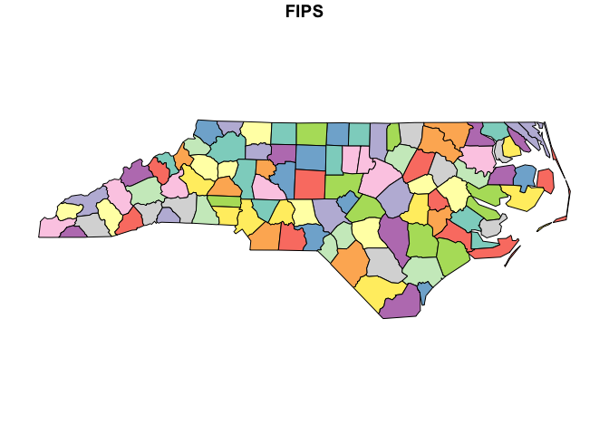
Now simplify using default parameters, then plot the simplified North Carolina counties:
nc_simp <- ms_simplify(nc_sf)
plot(nc_simp["FIPS"])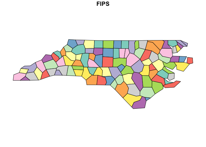
You can see that even at very high levels of simplification, the
mapshaper simplification algorithm preserves the topology, including
shared boundaries. The keep parameter specifies what
proportion of vertices to keep:
nc_very_simp <- ms_simplify(nc_sf, keep = 0.001)
plot(nc_very_simp["FIPS"])
Compare this to the output using sf::st_simplify, where
overlaps and gaps are evident:
nc_stsimp <- st_simplify(nc_sf, preserveTopology = TRUE, dTolerance = 10000) # dTolerance specified in meters
plot(nc_stsimp["FIPS"])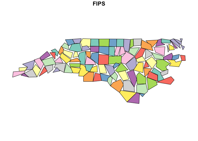
This time we’ll demonstrate the ms_innerlines
function:
nc_sf_innerlines <- ms_innerlines(nc_sf)
plot(nc_sf_innerlines)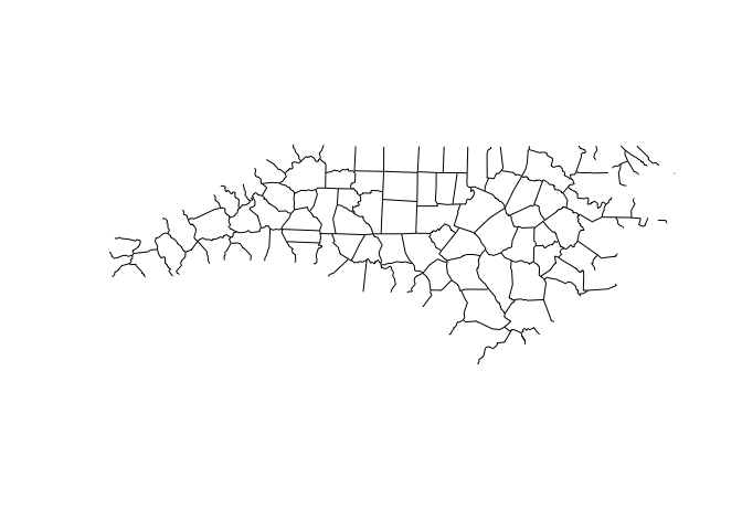
All of the functions are quite fast with geojson
character objects. They are slower with the sf and
Spatial classes due to internal conversion to/from json. If
you are going to do multiple operations on large sf
objects, it’s recommended to first convert to json using
geojsonsf::sf_geojson(), or
geojsonio::geojson_json(). All of the functions have the
input object as the first argument, and return the same class of object
as the input. As such, they can be chained together. For a totally
contrived example, using nc_sf as created above:
library(geojsonsf)
library(rmapshaper)
library(sf)

## First convert 'states' dataframe from geojsonsf pkg to json

nc_sf |>
  sf_geojson() |>
  ms_erase(bbox = c(-80, 35, -79, 35.5)) |> # Cut a big hole in the middle
  ms_dissolve() |> # Dissolve county borders
  ms_simplify(keep_shapes = TRUE, explode = TRUE) |> # Simplify polygon
  geojson_sf() |> # Convert to sf object
  plot(col = "blue") # plot
Sometimes if you are dealing with a very large spatial object in R,
rmapshaper functions will take a very long time or not work
at all. As of version 0.4.0, you can make use of the system
mapshaper library if you have it installed. This will allow
you to work with very large spatial objects.
First make sure you have mapshaper installed:
check_sys_mapshaper()
#> mapshaper version 0.6.113 is installed and on your PATH
#>                     mapshaper-xl
#> "/opt/homebrew/bin/mapshaper-xl"
If you get an error, you will need to install mapshaper. First install node (https://nodejs.org/en) and then install mapshaper in a command prompt with:
$ npm install -g mapshaperThen you can use the sys argument in any rmapshaper
function:
nc_simp_internal <- ms_simplify(nc_sf)
nc_simp_sys <- ms_simplify(nc_sf, sys = TRUE, sys_mem = 8) #sys_mem specifies the amount of memory to use in Gb.  It defaults to 8 if omitted.

par(mfrow = c(1, 2))
plot(st_geometry(nc_simp_internal), main = "internal")
plot(st_geometry(nc_simp_sys), main = "system")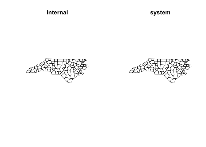
This package uses the V8 package to provide
an environment in which to run mapshaper’s javascript code in R. It
relies heavily on all of the great spatial packages that already exist
(especially sf), and the geojsonio and the
geojsonsf packages for converting between
geojson, sf and Spatial
object.
Thanks to timelyportfolio for helping me wrangle the javascript to the point where it works in V8. He also wrote the mapshaper htmlwidget, which provides access to the mapshaper web interface, right in your R session. We have plans to combine the two in the future.
Please note that this project is released with a Contributor Code of Conduct. By participating in this project you agree to abide by its terms.
MIT