README

Some survey participants tend to respond carelessly which complicates data analysis. This R package provides functions that make it easier to explore responses and identify those that may be problematic. This package implements two approaches to the problem of careless responses detection:
- rp.acors is based on the auto-correlation approach that allows for a probabilistic detection of repetitive patterns a in survey data. This function calculates auto-correlation coefficients for all lags up to the value defined by the max.lag parameter for each observation (respondent). Subsequently, it assigns a percentile value to each observation (respondent) based either on the highest absolute auto-correlation or the sum of absolute auto-correlations.
- rp.patterns takes a more mechanistic approach. It searches for repetitive patterns in the data using an iterative algorithm. Patterns are defined based on the data: if a sequence of values occurs more than once within an observation, it is considered a repetition. The algorithm counts the number of repetitions for each pattern length and then weighs this sum by the length of the pattern (longer patterns are assigned higher weight). The total score for each respondent is determined as the sum of scores achieved for each pattern length and is standardized to a value between 0 and 1.

Both approaches yield scores that serve as estimates of how problematic the observations potentially are (“suspicion” scores). However, no conclusions should be made without a closer inspection of the problematic responses. Any decision about removing or downweighing an observation should be based on visual inspection of the responses, the specifics of the instrument used to collect the data, researchers’ familiarity with the whole data set and the context of the data collection process.

In order to prevent bias, only questions with the same answer scales should be analyzed at one time, ideally. Analyzing responses on two scales with different number ranges together (e.g., answers on scale 1–5 and answers on scale 1–100) can bias the results to a great extent. See below for an example of how to analyze data from several questionnaires simultaneously. Questions with unique scales or answer options where repetitive response patterns are unlikely or even impossible to emerge, like questions about gender or education, should be excluded prior to screening.

Both core functions return an S4 object of class ResponsePatterns. The package offers several utility functions that allow to inspect to results of the analysis more closely:
- rp.summary (or, simply, summary) provides an overview of the object;
- rp.indices extracts indices and, optionally, coefficients, from the object;
- rp.select reorders observations and selects those equal of above a defined percentile;
- rp.save2csv exports indices and, optionally, coefficients and data into a CSV file;
- rp.hist plots a histogram of the main “suspicion” index (see the documentation for further details);
- rp.plot plots an individual response for easier visual inspection and allows for graphical formatting that eases this inspection;
- rp.plots2pdf exports a collection of individual plots into a PDF file.

Installation

install.packages("responsePatterns")

# install.packages("devtools")
devtools::install_github("trihacek/responsePatterns")

Examples

The package comes with an N = 100 data set (rp.simdata) that contains an ID variable (called “optional_ID”) and simulated responses to 20 items rated on a Likert-type scale ranging from 1 to 5. We use this data set to demonstrate the functionality of the package.

First, create a ResponsePatterns object that contains information about the potentially problematic patterns.

library(responsePatterns)
#> This is responsePatterns 0.1.1. Note: this is BETA software! Please mind that the package may not be stable and report any bugs! For questions and issues, please see github.com/trihacek/responsePatterns.
# Use auto-correlation screening to find patterns in the data
rp1 <- rp.acors(rp.simdata, max.lag = 5, id.var = "optional_ID")
# Alternatively, use an iterative mechanistic method for pattern detection
rp2 <- rp.patterns(rp.simdata, id.var = "optional_ID")

# Display a summary of the analysis
rp.summary(rp1)
#> --------------------------
#> Response Patterns Analysis
#> --------------------------
#> 
#> Method:  acors 
#> Number of variables:  20 
#> Number of observations:  100 
#> Limited to: min.lag=1, max.lag=5
#> Contains: full data set
#> Remove missing values:  FALSE 
#> Correlation method:  pearson 
#> Average max. auto-correlation:  0.42 
#> The modal lag of max. auto-correlation:  5 
#> Average number of failed auto-correlations:  0 
#> 
#> Tips
#>  - Use rp.indices() to extract max. auto-correlations and other indices
#>  - Use rp.select() to select cases for further exploration based on percentiles
#>  - Use rp.hist() to plot the distribution of max. auto-correlations
#>  - Use rp.plot() to plot individual responses for further exploration
#>  - Use rp.plots2pdf() to print a series of plots into a PDF file
#>  - Use rp.save2csv() to save results of the analysis into a CSV file

Second, select observations above the 90th (or any other) percentile for closer examination and extract (or export) the indices.

# Select observations above X percentile
rp.selected <- rp.select(rp1, percentile = 90)

# Extract indices
indices <- rp.indices(rp1, include.coefs = FALSE)
head(indices)
#>   sum.abs.ac max.abs.ac max.ac.lag n.failed.ac percentile
#> 1       1.14       0.42          3           0         54
#> 2       0.61       0.27          2           0         19
#> 3       0.51       0.25          2           0         14
#> 4       0.87       0.37          3           0         46
#> 5       0.24       0.08          4           0          1
#> 6       0.57       0.32          5           0         33


# Export indices into a CVS file
rp.save2csv(rp1)

# You may also plot a histogram of the 'suspicion' score to get an idea of what
# your data set looks like overall
rp.hist(rp1)

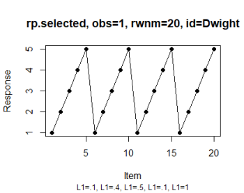
# Select the observation (see IMG 1)
rp.plot(rp.selected, obs = 1)

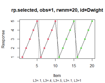
# Optionally, color the items based, for instance, on their positive vs.
# negative valence and display pagination of the questionnaire (see IMG 2)
rp.plot(rp.selected, obs = 1, groups = list(c(1:10), c(11:20)), page.breaks = c(5,
    10, 15))

# You may also export a collection of all plots into a PDF file (utilizing the
# same graphical arguments as the single rp.plot function)
rp.plots2pdf(rp.selected, groups = list(c(1:10), c(11:20)), page.breaks = c(5, 10,
    15))

library(magrittr)

rp.acors(rp.simdata, max.lag = 5, id.var = "optional_ID") %>%
    rp.select(percentile = 90) %>%
    rp.indices()

rp2 %>%
    rp.select(percentile = 80) %>%
    rp.plots2pdf()

Sometimes, we use multiple questionnaires in a survey. In such a case, we may wish to analyze the data from all questionnaires simultaneously. We do not recommend entering all data in a single analysis, since different questionnaires may use different rating scales and participants may change their style of responding. Instead, we recommend analyzing each questionnaire separately and then collate the results. To make this example easy, let’s imagine that the rp.simdata data set consists of data collected via four 5-item questionnaires.

# First, analyze each questionnaire separately
rp.a <- rp.acors(rp.simdata[, c(2:6)])
rp.b <- rp.acors(rp.simdata[, c(7:11)])
rp.c <- rp.acors(rp.simdata[, c(12:16)])
rp.d <- rp.acors(rp.simdata[, c(17:21)])

# Second, collate the percentiles
percentiles <- as.data.frame(cbind(rp.simdata$optional_ID, rp.indices(rp.a)$percentile,
    rp.indices(rp.b)$percentile, rp.indices(rp.c)$percentile, rp.indices(rp.d)$percentile))

# Choose a cutoff, let's say the 95th percentile, and count how many times each
# person exceededs this cutoff (here, we chose the 80th percentile for
# demonstration reasons, because the 95th percentile would not yield any
# suspicious responses)
percentile.cutoff <- 80
percentiles$sum <- rowSums(percentiles > percentile.cutoff)

# Decide on how many times a respondent must be placed above the percentile
# cutoff score to be considered problematic. Then, select potentially
# problematic responses
sum.cutoff <- 2
IDs <- percentiles[percentiles$sum >= sum.cutoff, 1]

# Create a loop to output these responses into a PDF file for further
# inspection.
pdf(file = "rp_plots_screening.pdf", width = 10, height = 6)
for (i in 1:length(IDs)) {
    layout(matrix(1:4, ncol = 2, nrow = 2, byrow = T))
    rp.plot(rp.a, obs = i)
    rp.plot(rp.b, obs = i)
    rp.plot(rp.c, obs = i)
    rp.plot(rp.d, obs = i)
}
dev.off()

# Then, open the PDF file and explore the responses to decide if any of them
# should be removed from further analysis.