


![]()
![]()
Version 1.1.3 built 2022-05-02 with R 4.2.0 (development version not on CRAN).
The package provides data sets (internal .rda and in
CSV-format in
/extdata/) supporting users in a black-box performance
qualification (PQ) of their software installations. Users can analyze
own data imported from
CSV- and Excel-files
(in xlsx or the legacy xls format). The
methods given by the EMA
for reference-scaling of
HVD(P)s,
i.e., Average Bioequivalence with Expanding Limits
(ABEL)1,2 are implemented.
Potential influence of
outliers on the variability of the reference can be assessed by box
plots of studentized and standardized residuals as suggested at a joint
EGA/EMA
workshop.3
Health Canada’s
approach4 requiring a mixed-effects
model is approximated by intra-subject contrasts.
Direct widening of the acceptance range as recommended by the Gulf
Cooperation Council5 (Bahrain,
Kuwait, Oman, Qatar, Saudi Arabia, United Arab Emirates) is provided as
well.
In full replicate designs the variability of test and reference
treatments can be assessed by
swT/swR and the upper confidence
limit of σwT/σwR. This was
required in a pilot phase by the
WHO but lifted in 2021;
reference-scaling of AUC is acceptable if the protocol is
submitted to the
PQT/MED.6
Called internally by functions method.A() and
method.B(). A linear model of log-transformed
pharmacokinetic (PK) responses and effects
sequence, subject(sequence),
period
where all effects are fixed (i.e., by an
ANOVA). Estimated by the
function lm() of package stats.
modCVwR <- lm(log(PK) ~ sequence + subject%in%sequence + period,
                        data = data[data$treatment == "R", ])
modCVwT <- lm(log(PK) ~ sequence + subject%in%sequence + period,
data = data[data$treatment == "T", ])Called by function method.A(). A linear model of
log-transformed PK responses and
effects
sequence, subject(sequence),
period, treatment
where all effects are fixed (e.g., by an
ANOVA). Estimated by the
function lm() of package stats.
modA <- lm(log(PK) ~ sequence + subject%in%sequence + period + treatment,
data = data)Called by function method.B(). A linear model of
log-transformed PK responses and
effects
sequence, subject(sequence),
period, treatment
where subject(sequence) is a random effect and all
others are fixed.
Three options are provided:
lmer() of package
lmerTest. method.B(..., option = 1) employs
Satterthwaite’s approximation of the degrees of freedom equivalent to
SAS’ DDFM=SATTERTHWAITE, Phoenix WinNonlin’s
Degrees of Freedom Satterthwaite, and Stata’s
dfm=Satterthwaite. Note that this is the only available
approximation in SPSS.modB <- lmer(log(PK) ~ sequence + period + treatment + (1|subject),
data = data)lme() of package
nlme. method.B(..., option = 2) employs
degrees of freedom equivalent to SAS’ DDFM=CONTAIN, Phoenix
WinNonlin’s Degrees of Freedom Residual, STATISTICA’s
GLM containment, and Stata’s dfm=anova.
Implicitly preferred according to the
EMA’s
Q&A document and hence,
the default of the function.modB <- lme(log(PK) ~ sequence + period + treatment, random = ~1|subject,
data = data)lmer() of package
lmerTest. method.B(..., option = 3) employs
the Kenward-Roger approximation equivalent to Stata’s
dfm=Kenward Roger (EIM) and SAS’
DDFM=KENWARDROGER(FIRSTORDER) i.e., based on the
expected information matrix. Note that SAS with
DDFM=KENWARDROGER and JMP calculate Satterthwaite’s
[sic] degrees of freedom and apply the Kackar-Harville
correction, i.e., based on the observed information
matrix.modB <- lmer(log(PK) ~ sequence + period + treatment + (1|subject),
data = data)Called by function ABE(). The model is identical to Method A. Conventional BE limits (80.00 – 125.00%)
are employed by default. Tighter limits (90.00 – 111.11%) for narrow
therapeutic index drugs
(EMA and others) or wider
limits (75.00 – 133.33%) for Cmax according to the
guideline of South Africa7 can be
specified.
TRTR | RTRT
TRRT | RTTR
TTRR | RRTT
TRTR | RTRT | TRRT | RTTR
TRRT | RTTR | TTRR | RRTT
TRT | RTR
TRR | RTT
TR | RT | TT | RR (Balaam’s design; not
recommended due to poor power characteristics)
TRR | RTR | RRT
TRR | RTR (Extra-reference design; biased in the
presence of period effects, not recommended)
Details about the reference datasets:
help("data", package = "replicateBE")
?replicateBE::data
Results of the 30 reference datasets agree with ones obtained in SAS (v9.4), Phoenix WinNonlin (v6.4 – v8.3.4.295), STATISTICA (v13), SPSS (v22.0), Stata (v15.0), and JMP (v10.0.2).8
library(replicateBE) # attach the package
res <- method.A(verbose = TRUE, details = TRUE,
                print = FALSE, data = rds01)
#
# Data set DS01: Method A by lm()
# ───────────────────────────────────
# Type III Analysis of Variance Table
#
# Response: log(PK)
#                   Df   Sum Sq  Mean Sq  F value     Pr(>F)
# sequence           1   0.0077 0.007652  0.00268  0.9588496
# period             3   0.6984 0.232784  1.45494  0.2278285
# treatment          1   1.7681 1.768098 11.05095  0.0010405
# sequence:subject  75 214.1296 2.855061 17.84467 < 2.22e-16
# Residuals        217  34.7190 0.159995
#
# treatment T – R:
#   Estimate Std. Error    t value   Pr(>|t|)
# 0.14547400 0.04650870 3.12788000 0.00200215
# 217 Degrees of Freedom
cols <- c(12, 17:21)           # extract relevant columns
# cosmetics: 2 decimal places acc. to the GL
tmp  <- data.frame(as.list(sprintf("%.2f", res[cols])))
names(tmp) <- names(res)[cols]
tmp  <- cbind(tmp, res[22:24]) # pass|fail
print(tmp, row.names = FALSE)
#  CVwR(%)  L(%)   U(%) CL.lo(%) CL.hi(%)  PE(%)   CI  GMR   BE
# 46.96 71.23 140.40 107.11 124.89 115.66 pass pass passres <- method.B(option = 1, verbose = TRUE, details = TRUE,
print = FALSE, data = rds01)
#
# Data set DS01: Method B (option = 1) by lmer()
# ──────────────────────────────────────────────
# Response: log(PK)
# Type III Analysis of Variance Table with Satterthwaite's method
# Sum Sq Mean Sq NumDF DenDF F value Pr(>F)
# sequence 0.001917 0.001917 1 74.7208 0.01198 0.9131536
# period 0.398078 0.132693 3 217.1188 0.82881 0.4792840
# treatment 1.579332 1.579332 1 216.9386 9.86464 0.0019197
#
# treatment T – R:
# Estimate Std. Error t value Pr(>|t|)
# 0.1460900 0.0465130 3.1408000 0.0019197
# 216.939 Degrees of Freedom (equivalent to SAS’ DDFM=SATTERTHWAITE)
cols <- c(12, 17:21)
tmp <- data.frame(as.list(sprintf("%.2f", res[cols])))
names(tmp) <- names(res)[cols]
tmp <- cbind(tmp, res[22:24])
print(tmp, row.names = FALSE)
# CVwR(%) L(%) U(%) CL.lo(%) CL.hi(%) PE(%) CI GMR BE
# 46.96 71.23 140.40 107.17 124.97 115.73 pass pass passres <- method.B(option = 3, ola = TRUE, verbose = TRUE,
details = TRUE, print = FALSE, data = rds01)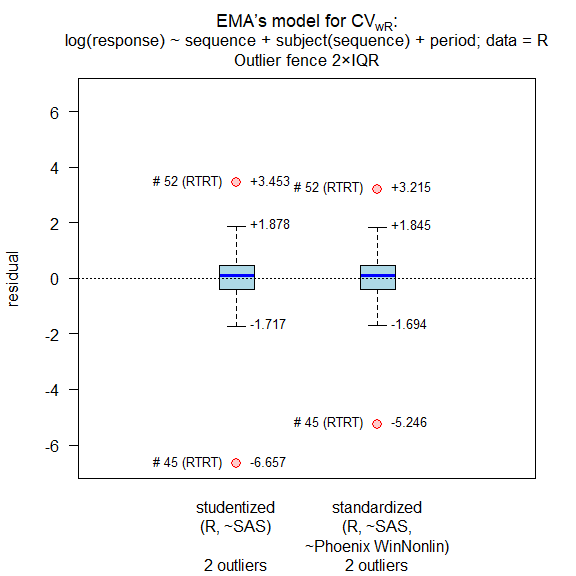
#
# Outlier analysis
#  (externally) studentized residuals
#  Limits (2×IQR whiskers): -1.717435, 1.877877
#  Outliers:
#  subject sequence  stud.res
#       45     RTRT -6.656940
#       52     RTRT  3.453122
#
#  standarized (internally studentized) residuals
#  Limits (2×IQR whiskers): -1.69433, 1.845333
#  Outliers:
#  subject sequence stand.res
#       45     RTRT -5.246293
#       52     RTRT  3.214663
#
# Data set DS01: Method B (option = 3) by lmer()
# ──────────────────────────────────────────────
# Response: log(PK)
# Type III Analysis of Variance Table with Kenward-Roger's method
#             Sum Sq  Mean Sq NumDF    DenDF F value    Pr(>F)
# sequence  0.001917 0.001917     1  74.9899 0.01198 0.9131528
# period    0.398065 0.132688     3 217.3875 0.82878 0.4792976
# treatment 1.579280 1.579280     1 217.2079 9.86432 0.0019197
#
# treatment T – R:
#   Estimate Std. Error    t value   Pr(>|t|)
#  0.1460900  0.0465140  3.1408000  0.0019197
# 217.208 Degrees of Freedom (equivalent to Stata’s dfm=Kenward Roger EIM)
cols <- c(27, 31:32, 19:21)
tmp  <- data.frame(as.list(sprintf("%.2f", res[cols])))
names(tmp) <- names(res)[cols]
tmp  <- cbind(tmp, res[22:24])
print(tmp, row.names = FALSE)
#  CVwR.rec(%) L.rec(%) U.rec(%) CL.lo(%) CL.hi(%)  PE(%)   CI  GMR   BE
# 32.16 78.79 126.93 107.17 124.97 115.73 pass pass passres <- method.A(regulator = "GCC", details = TRUE,
print = FALSE, data = rds01)
cols <- c(12, 17:21)
tmp <- data.frame(as.list(sprintf("%.2f", res[cols])))
names(tmp) <- names(res)[cols]
tmp <- cbind(tmp, res[22:24])
print(tmp, row.names = FALSE)
# CVwR(%) L(%) U(%) CL.lo(%) CL.hi(%) PE(%) CI GMR BE
# 46.96 75.00 133.33 107.11 124.89 115.66 pass pass passres <- ABE(theta1 = 0.75, details = TRUE,
print = FALSE, data = rds01)
tmp <- data.frame(as.list(sprintf("%.2f", res[12:17])))
names(tmp) <- names(res)[12:17]
tmp <- cbind(tmp, res[18])
print(tmp, row.names = FALSE)
# CVwR(%) BE.lo(%) BE.hi(%) CL.lo(%) CL.hi(%) PE(%) BE
# 46.96 75.00 133.33 107.11 124.89 115.66 passres <- ABE(theta1 = 0.90, details = TRUE,
print = FALSE, data = rds05)
cols <- c(13:17)
tmp <- data.frame(as.list(sprintf("%.2f", res[cols])))
names(tmp) <- names(res)[cols]
tmp <- cbind(tmp, res[18])
print(tmp, row.names = FALSE)
# BE.lo(%) BE.hi(%) CL.lo(%) CL.hi(%) PE(%) BE
# 90.00 111.11 103.82 112.04 107.85 failThe package requires R ≥3.5.0. However, for the Kenward-Roger
approximation method.B(..., option = 3) R ≥3.6.0 is
required.
install.packages("replicateBE", repos = "https://cloud.r-project.org/")To use the development version, please install the released version from CRAN first to get its dependencies right (readxl ≥1.0.0, PowerTOST ≥1.5.3, lmerTest, nlme, pbkrtest).
You need tools for building R packages from sources on your machine. For Windows users:
devtools and build the development version
by:install.packages("devtools", repos = "https://cloud.r-project.org/")
devtools::install_github("Helmut01/replicateBE")Inspect this information for reproducibility. Of particular importance are the versions of R and the packages used to create this workflow. It is considered good practice to record this information with every analysis.
options(width = 66)
print(sessionInfo(), locale = FALSE)
# R version 4.2.0 (2022-04-22 ucrt)
# Platform: x86_64-w64-mingw32/x64 (64-bit)
# Running under: Windows 10 x64 (build 22000)
#
# Matrix products: default
#
# attached base packages:
# [1] stats     graphics  grDevices utils     datasets  methods
# [7] base
#
# other attached packages:
# [1] replicateBE_1.1.3
#
# loaded via a namespace (and not attached):
#  [1] tidyselect_1.1.2    xfun_0.30           purrr_0.3.4
#  [4] splines_4.2.0       lmerTest_3.1-3      lattice_0.20-45
#  [7] colorspace_2.0-3    vctrs_0.4.1         generics_0.1.2
# [10] htmltools_0.5.2     yaml_2.3.5          utf8_1.2.2
# [13] rlang_1.0.2         pillar_1.7.0        nloptr_2.0.0
# [16] glue_1.6.2          PowerTOST_1.5-4     readxl_1.4.0
# [19] lifecycle_1.0.1     stringr_1.4.0       munsell_0.5.0
# [22] gtable_0.3.0        cellranger_1.1.0    mvtnorm_1.1-3
# [25] evaluate_0.15       knitr_1.39          fastmap_1.1.0
# [28] parallel_4.2.0      pbkrtest_0.5.1      fansi_1.0.3
# [31] highr_0.9           broom_0.8.0         Rcpp_1.0.8.3
# [34] backports_1.4.1     scales_1.2.0        lme4_1.1-29
# [37] TeachingDemos_2.12  ggplot2_3.3.5       digest_0.6.29
# [40] stringi_1.7.6       dplyr_1.0.8         numDeriv_2016.8-1.1
# [43] grid_4.2.0          cli_3.3.0           tools_4.2.0
# [46] magrittr_2.0.3      tibble_3.1.6        tidyr_1.2.0
# [49] crayon_1.5.1        pkgconfig_2.0.3     MASS_7.3-57
# [52] ellipsis_0.3.2      Matrix_1.4-1        minqa_1.2.4
# [55] rmarkdown_2.14      rstudioapi_0.13     cubature_2.0.4.4
# [58] R6_2.5.1            boot_1.3-28         nlme_3.1-157
# [61] compiler_4.2.0Helmut Schütz (author) ORCID iD
Michael Tomashevskiy (contributor)
Detlew Labes (contributor) ORCID iD
Package offered for Use without any Guarantees and Absolutely No Warranty. No Liability is accepted for any Loss and Risk to Public Health Resulting from Use of this R-Code.
1.
EMA. EMA/582648/2016.
Annex I. London. 21 September 2016. Online
↩︎
2.
EMA,
CHMP.
CPMP/EWP/QWP/1401/98 Rev. 1/ Corr **. London. 20 January 2010. Online.
↩︎
3.
EGA.
Revised EMA Bioequivalence Guideline. Questions & Answers.
London. June 2010. Online
↩︎
4. Health Canada. Guidance
Document. Conduct and Analysis of Comparative Bioavailability
Studies. Ottawa. 2018/06/08. Online.
↩︎
5. Executive Board of the
Health Ministers’ Council for
GCC States. The GCC
Guidelines for Bioequivalence. Version 3.0. May 2021. Online.
↩︎
6.
WHO. Application of
reference-scaled criteria for AUC in bioequivalence studies conducted
for submission to
PQT/MED.
Geneva. 02 July 2021. Online.
↩︎
7.
MCC. Registration of
Medicines. Biostudies. Pretoria. June 2015. Online.
↩︎
8. Schütz H, Tomashevskiy M,
Labes D, Shitova A, González-de la Parra M, Fuglsang A. Reference
Datasets for Studies in a Replicate Design Intended for Average
Bioequivalence with Expanding Limits. AAPS J. 2020; 22(2):
Article 44. doi:10.1208/s12248-020-0427-6.
↩︎
9.
EMA. EMA/582648/2016.
Annex II. London. 21 September 2016. Online.
↩︎
10. Shumaker RC, Metzler CM.
The Phenytoin Trial is a Case Study of ‘Individual’
Bioequivalence. Drug Inf J. 1998; 32(4): 1063–72. doi:10.1177/009286159803200426.
↩︎