randomForestVIP

The goal of randomForestVIP is to tune and select a good Random Forest model based on the accuracy and variable importance metrics associated with each model. To accomplish this, functions are available to tabulate and plot results designed to help the user select an optimal model.

This package contains functions for assessing variable relations and associations prior to modeling with a Random Forest algorithm (although these are relevant for any predictive model). Metrics such as partial correlations and variance inflation factors are tabulated as well as plotted for the user using the functions partial_cor and robust_vifs.

The function mtry_compare is available for tuning the hyper-parameter mtry based on model performance and variable importance metrics. This grid-search technique provides tables and plots showing the effect of mtry on each of the assessment metrics. It also returns each of the evaluated models to the user.

The package also provides superior ggplot2 variable importance plots for individual models using the function ggvip. This function is a highly aesthetic and editable improvement upon the function randomForest::varImpPlot and other basic importance graphics.

All of the plots generated by these functions are developed with ggplot2 techniques so that the user has the ability to edit and improve further upon the plots.

For methodology see “Contributions to Random Forest Variable Importance with Applications in R” https://digitalcommons.usu.edu/etd/8587/.

Installation

You can install the released version of randomForestVIP from CRAN with:

install.packages("randomForestVIP")

You can install the development version of randomForestVIP from GitHub with:

# install.packages("devtools")
devtools::install_github("KelvynBladen/randomForestVIP")

You can view R package’s source code on GitHub: https://github.com/KelvynBladen/randomForestVIP

Example

library(randomForestVIP)
library(MASS)
library(EZtune)

To introduce the functionality of randomForestVIP, we look at modeling the Boston housing data (found in the MASS package). We want to build a Random Forest model with a view towards both accuracy and interpretability. We begin by running some preliminary diagnostics on our data.

set.seed(1234)

pcs <- partial_cor(medv ~ ., data = Boston, model = lm)
pcs$plot_y_part_cors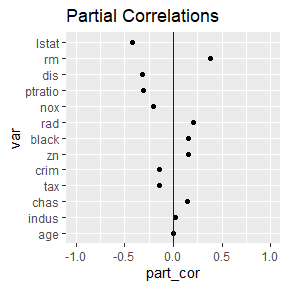

rv <- robust_vifs(medv ~ ., data = Boston, model = lm)
rv$plot_lin_vifs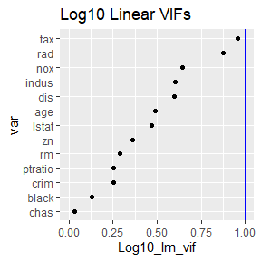

These functions assess concerns with collinearity. Notice that the VIFs from robust_vifs are all less than 10. The partial correlations with the response from partial_cor are a type of pseudo-importance assessing the importance each variable does not share with the others. Now we tune our model by assessing four different mtry values in the mtry_compare function.

set.seed(1)
m <- mtry_compare(medv ~ .,
  data = Boston, sqrt = TRUE,
  mvec = c(1, 4, 9, 13), num_var = 7
)
m$gg_model_errors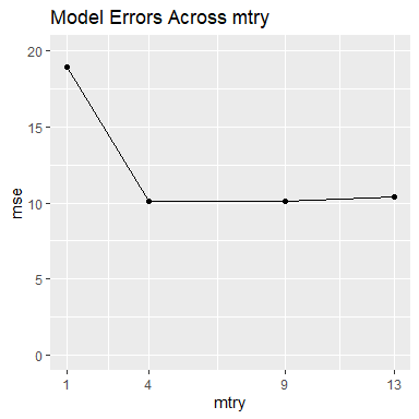

m$model_errors
#>   mtry      mse
#> 1    1 18.96051
#> 2    4 10.11247
#> 3    9 10.13187
#> 4   13 10.36482

According to the accuracy plot and table above, our best choice is when mtry is 4. However, the accuracy for the best model is notably only slightly better than the models with mtry set to 9 and 13. We now look at the variable importance metrics across the different models.

m$gg_var_imp_error

The top two variables are consistently identified as more important than the other variables and their order remains unchanged across mtry. However, the variables ‘nox’ and ‘dis’ switch order as mtry increases. Pollution (nox) has a strong negative correlation with distance to employment centers (dis). This makes sense if the employment centers are responsible for much of the pollution. If many home buyers consider distance to work more important than pollution when selecting a house, ‘dis’ is more likely to be a causal driver of price than ‘nox’. By this reasoning, the model where mtry is 9 appears to be superior to the model where mtry is 4, despite mtry of 4 yielding slightly more accurate results.

We now take our selected model and build individual importance plots for it using ggvip.

g <- ggvip(m$rf9, num_var = 7)$both_vips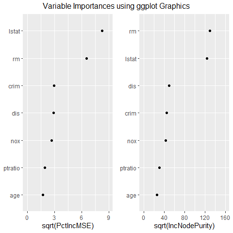

The plot above resembles a standard variable importance plot, but possesses superior tick labels and editing capabilities for the analyst.

We have used the randomForestVIP package to tune a strong model for prediction and with reasonably useful importance values. This was accomplished by assessing variable importance and accuracy metrics across the hyper-parameter mtry.