![]()
The goal of quarks is to enable the user to compute
Value at Risk (VaR) and Expected Shortfall (ES) by means of various
types of historical simulation. Currently plain historical simulation as
well as age-, volatility-weighted- and filtered historical simulation
are implemented in quarks. Volatility weighting can be
carried out via an exponentially weighted moving average (EWMA) model or
other GARCH-type models.
You can install the released version of quarks from CRAN with:
install.packages("quarks")The data set DAX, which is implemented in the
quarks package, contains daily financial data of the German
stock index DAX from January 2000 to December 2021 (currency in EUR). In
the following examples of the (out-of-sample) one-step forecasts of the
97.5-VaR (red line) and the corresponding ES (green
line) are illustrated. Exceedances are indicated by the colored
circles.
# Calculating the returns
prices <- DAX$price.close
returns <- diff(log(prices))
Example 1 - plain historical simulation
results1 <- rollcast(x = returns, p = 0.975, method = 'plain', nout = 250,
                     nwin = 250)
#>
#> Calculations completed.
results1
#>
#> --------------------------------------------
#> |              Specifications              |
#> --------------------------------------------
#>  Out-of-sample size:    250
#>  Rolling window size:   250
#>  Bootstrap sample size: N/A
#>  Confidence level:      97.5 %
#>  Method:                Plain
#>  Model:                 EWMA
#> --------------------------------------------
#> |           Forecast performance           |
#> --------------------------------------------
#>  Out-of-sample losses exceeding VaR
#>
#>  Number of breaches:    4
#> --------------------------------------------
#>  Out-of-sample losses exceeding ES
#>
#>  Number of breaches:    1
#> --------------------------------------------
Visualize your results with the plot method implemented in
quarks.
plot(results1)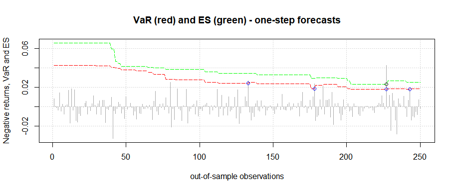
Example 2 - age weighted historical simulation
results2 <- rollcast(x = returns, p = 0.975, method = 'age', nout = 250,
                     nwin = 250)
#>
#> Calculations completed.
results2
#>
#> --------------------------------------------
#> |              Specifications              |
#> --------------------------------------------
#>  Out-of-sample size:    250
#>  Rolling window size:   250
#>  Bootstrap sample size: N/A
#>  Confidence level:      97.5 %
#>  Method:                Age Weighting
#>  Model:                 EWMA
#> --------------------------------------------
#> |           Forecast performance           |
#> --------------------------------------------
#>  Out-of-sample losses exceeding VaR
#>
#>  Number of breaches:    5
#> --------------------------------------------
#>  Out-of-sample losses exceeding ES
#>
#>  Number of breaches:    4
#> --------------------------------------------plot(results2)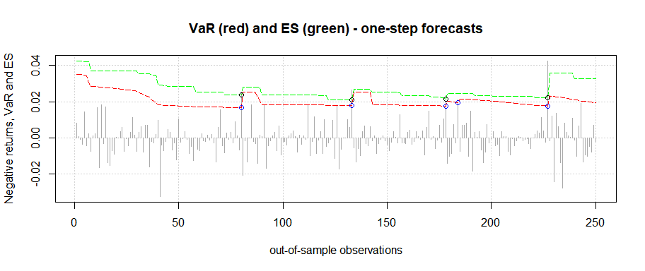
Example 3 - volatility weighted historical simulation - EWMA
results3 <- rollcast(x = returns, p = 0.975, model = 'EWMA',
                     method = 'vwhs', nout = 250, nwin = 250)
#>
#> Calculations completed.
results3
#>
#> --------------------------------------------
#> |              Specifications              |
#> --------------------------------------------
#>  Out-of-sample size:    250
#>  Rolling window size:   250
#>  Bootstrap sample size: N/A
#>  Confidence level:      97.5 %
#>  Method:                Volatility Weighting
#>  Model:                 EWMA
#> --------------------------------------------
#> |           Forecast performance           |
#> --------------------------------------------
#>  Out-of-sample losses exceeding VaR
#>
#>  Number of breaches:    4
#> --------------------------------------------
#>  Out-of-sample losses exceeding ES
#>
#>  Number of breaches:    3
#> --------------------------------------------plot(results3)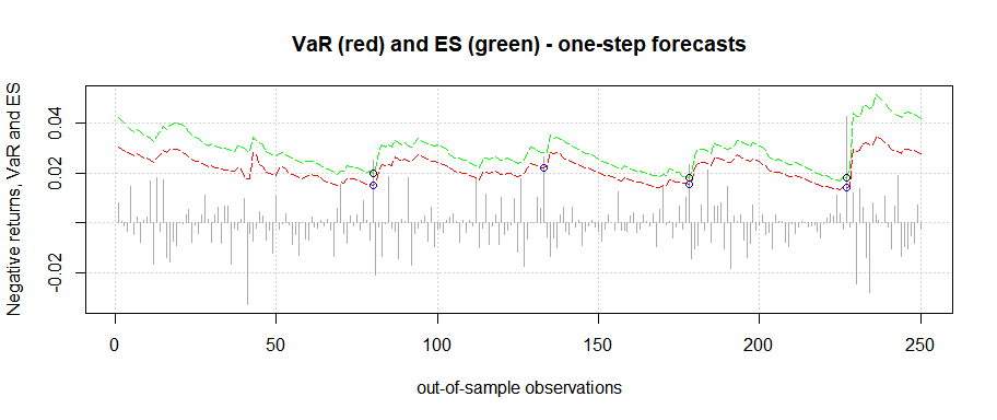
Example 4 - filtered historical simulation - GARCH
set.seed(12345)
results4 <- rollcast(x = returns, p = 0.975, model = 'GARCH',
                     method = 'fhs', nout = 250, nwin = 250, nboot = 10000)
#>
#> Calculations completed.
results4
#>
#> --------------------------------------------
#> |              Specifications              |
#> --------------------------------------------
#>  Out-of-sample size:    250
#>  Rolling window size:   250
#>  Bootstrap sample size: 10000
#>  Confidence level:      97.5 %
#>  Method:                Filtered
#>  Model:                 sGARCH
#> --------------------------------------------
#> |           Forecast performance           |
#> --------------------------------------------
#>  Out-of-sample losses exceeding VaR
#>
#>  Number of breaches:    5
#> --------------------------------------------
#>  Out-of-sample losses exceeding ES
#>
#>  Number of breaches:    2
#> --------------------------------------------plot(results4)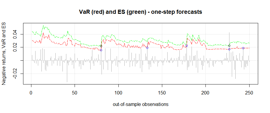
To assess the performance of these methods one might apply backtesting.
For instance, by employing the Traffic Light Test, Coverage Tests or by means of Loss Function.
Example 5 - Traffic Light Test
# Calculating the returns
prices <- SP500$price.close
returns <- diff(log(prices))

results <- rollcast(x = returns, p = 0.99, model = 'GARCH',
                     method = 'vwhs', nout = 250, nwin = 500)
#>
#> Calculations completed.
trftest(results)
#>
#> --------------------------------------------
#> |            Traffic Light Test            |
#> --------------------------------------------
#>  Method: Volatility Weighting
#>  Model:  sGARCH
#> --------------------------------------------
#> |       Traffic light zone boundaries      |
#> --------------------------------------------
#>  Zone         Probability
#>  Green zone:  p < 95%
#>  Yellow zone: 95% <= p < 99.99%
#>  Red zone:    p >= 99.99%
#> --------------------------------------------
#> |         Test result - 99%-VaR            |
#> --------------------------------------------
#>  Number of violations: 3
#>
#>  p = 0.7581: Green zone
#> --------------------------------------------
Example 6 - Coverage Tests
# Calculating the returns
prices <- HSI$price.close
returns <- diff(log(prices))

results <- rollcast(x = returns, p = 0.99, model = 'GARCH',
                     method = 'vwhs', nout = 250, nwin = 500)
#>
#> Calculations completed.
cvgtest(results, conflvl = 0.95)
#>
#> --------------------------------------------
#> |               Test results               |
#> --------------------------------------------
#>  Method: Volatility Weighting
#>  Model:  sGARCH
#> --------------------------------------------
#> |        Unconditional coverage test       |
#> --------------------------------------------
#> H0: w = 0.99
#>
#> p_[uc] = 0.758
#>
#> Decision: Fail to reject H0
#> --------------------------------------------
#> |            Independence test             |
#> --------------------------------------------
#> H0: w_[00] = w_[10]
#>
#> p_[ind] = 0.0196
#>
#> Decision: Reject H0
#> --------------------------------------------
#> |         Conditional coverage test        |
#> --------------------------------------------
#> H0: w_[00] = w_[10] = 0.99
#>
#> p_[cc] = 0.0625
#>
#> Decision: Fail to reject H0
#> --------------------------------------------
Example 7 - Loss Functions
# Calculating the returns
prices <- FTSE100$price.close
returns <- diff(log(prices))

results <- rollcast(x = returns, p = 0.99, model = 'GARCH',
                     method = 'vwhs', nout = 250, nwin = 500)
#>
#> Calculations completed.
lossfun(results)
#>
#> Please note that the following results are multiplied with 10000.
#> $lossfun1
#> [1] 2.27884
#>
#> $lossfun2
#> [1] 10.84525
#>
#> $lossfun3
#> [1] 10.99533
#>
#> $lossfun4
#> [1] 10.2165In quarks ten functions are available.
Functions - version 1.1.3:
cvgtest: Applies various coverage tests to Value at
Riskewma: Estimates volatility of a return series by means
of an exponentially weighted moving averagefhs: Calculates univariate Value at Risk and Expected
Shortfall by means of filtered historical simulationhs: Computes Value at Risk and Expected Shortfall by
means of plain and age-weighted historical simulationlossfun: Calculates of loss functions of ESplop: Profit & Loss operator function; Calculates
weighted portfolio returns or lossesrollcast: Computes rolling one-step-ahead forecasts of
Value at Risk and Expected ShortfallrunFTS: Starts a shiny application for downloading data
from Yahoo Financetrftest: Applies the Traffic Light Test to Value at
Riskvwhs: Calculates univariate Value at Risk and Expected
Shortfall by means of volatility weighted historical simulationFor further information on each of the functions, we refer the user to the manual or the package documentation.
DAX: Daily financial time series data of the German
Stock Market Index (DAX) from January 2000 to December 2021DJI: Daily financial time series data of the Dow Jones
Industrial Average (DJI) from January 2000 to December 2021FTSE100: Daily financial time series data of the
Financial Times Stock Exchange Index (FTSE) from January 2000 to
December 2021HSI: Daily financial time series data of the Hang Seng
Index (HSI) from January 2000 to December 2021NIK225: Daily financial time series data of the Nikkei
Heikin Kabuka Index (NIK) from January 2000 to December 2021SP500: Daily financial time series data of Standard and
Poor`s (SP500) from January 2000 to December 2021