![]()
![]()
![]()
![]()
nuggets is a package for R statistical computing
environment providing a framework for systematic exploration of
association rules (Agrawal (1994)),
contrast patterns (Chen (2022)),
emerging patterns (Dong (1999)),
subgroup discovery (Atzmueller (2015)), and
conditional correlations (Hájek (1978)).
User-defined functions may also be supplied to guide custom pattern
searches.
Supports both crisp (Boolean) and fuzzy data. Generates candidate conditions expressed as elementary conjunctions, evaluates them on a dataset, and inspects the induced sub-data for statistical, logical, or structural properties such as associations, correlations, or contrasts. Includes methods for visualization of logical structures and supports interactive exploration through integrated Shiny applications.
A lot of effort has been put into optimizing the performance of the package, especially for dense datasets. The core algorithms are implemented in C++ and use single-instruction multiple-data (SIMD) operations to speed up the operations.
On a randomly generated dataset with 1 million rows and 15 columns, association rules with at most 5 items in the antecedent, a support above 0.001, and a confidence above 0.5 were searched. The total times, including reading the data from the CSV file, searching for rules, and writing the result back to CSV, on a Linux desktop computer with standard installations of the packages, were as follows:
nuggets (R, boolean logic): 1.4 sarules - ECLAT (R, boolean logic): 2.9
sarules - Apriori (R, boolean logic): 3.3
sFuzzy variant of association rules, which is much more computationally intensive:
nuggets (R, fuzzy logic): 12.0 sFor comparison, two Python libraries performed as follows:
cleverminer (Python, boolean logic): 1m
15.0smlxtend (Python, boolean logic, frequent itemsets
only): 4h 11m 22.5sRead the full documentation of the nuggets package.
To install the stable version of nuggets from CRAN, type
the following command within the R session:
install.packages("nuggets", dependencies = TRUE)You can also install the development version of nuggets
from GitHub with:
install.packages("devtools")
devtools::install_github("beerda/nuggets")
To start using the package, load it to the R session with:
library(nuggets)The following example demonstrates how to use nuggets to
find association rules in the built-in mtcars dataset:
# Preprocess: dichotomize and fuzzify numeric variables
cars <- mtcars |>
    partition(cyl, vs:gear, .method = "dummy") |>
    partition(carb, .method = "crisp", .breaks = c(0, 3, 10)) |>
    partition(mpg, disp:qsec, .method = "triangle", .breaks = 3)

# Search for associations among conditions
rules <- dig_associations(cars,
                          antecedent = everything(),
                          consequent = everything(),
                          max_length = 4,
                          min_support = 0.1)

# Add various interest measures
rules <- add_interest(rules)

# Explore the found rules interactively
explore(rules, cars)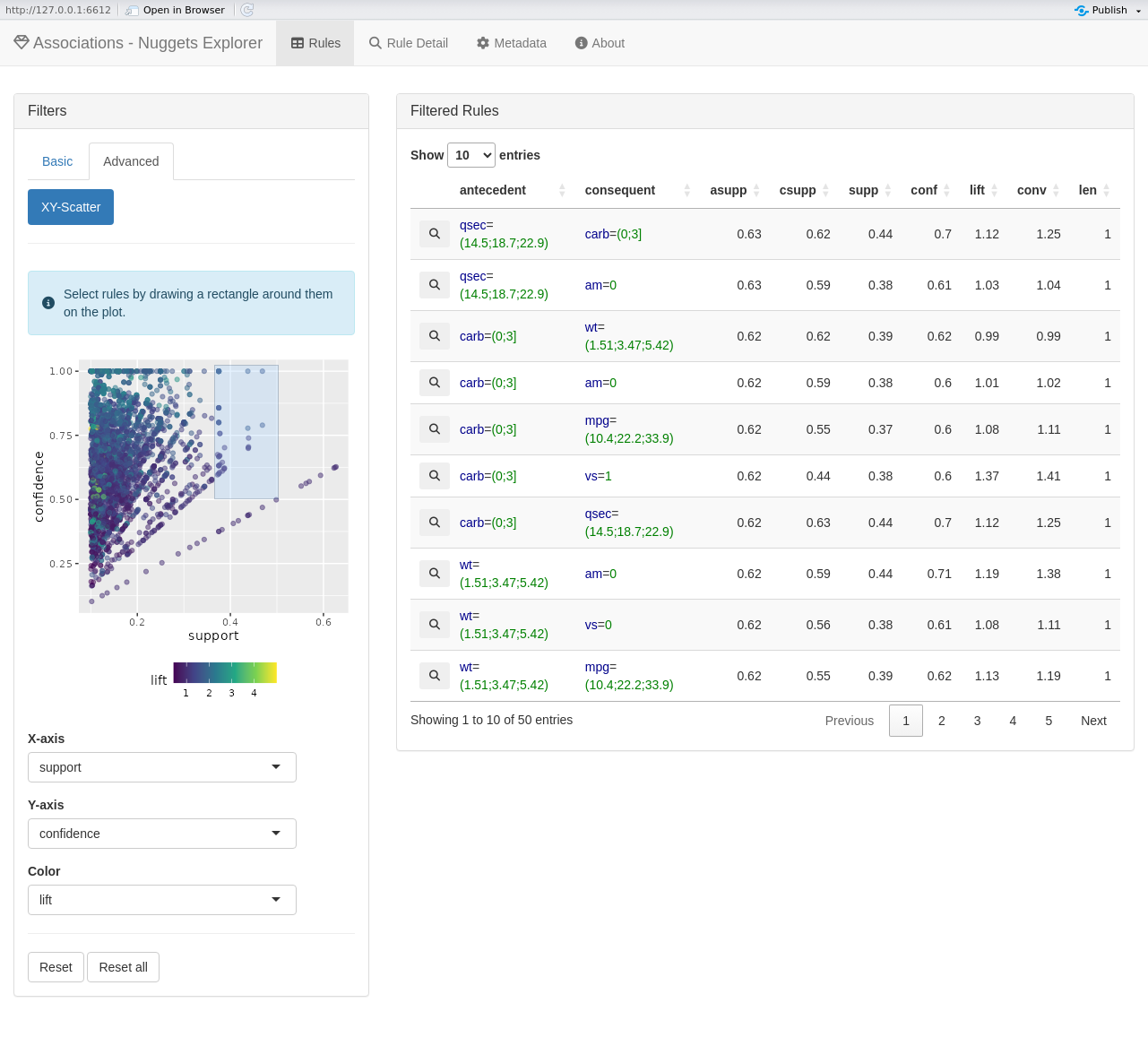
Contributions, suggestions, and bug reports are welcome. Please submit issues on GitHub.
This package is licensed under the GPL-3 license.
It includes third-party code licensed under BSD-2-Clause,
BSD-3-Clause, and GPL-2 or later licenses. See
inst/COPYRIGHTS for details.