mwa is a flexible methodological framework designed to
analyze causal relationships in spatially and temporally referenced
data. The study of political violence, in particular, has benefited in
recent years from a rapid increase in the availability of such data
sets. While progress has been made in relating conflict intensity to
geographic conditions, more complex endogenous mechanisms that drive
conflict at the micro-level remain largely elusive to quantitative
analysis. To fill this gap, we introduce a novel approach to causal
inference in disaggregated event data that combines two techniques for
ensuring robust and clean causal inference: sliding spatiotemporal
windows and statistical matching.
Specific types of events might affect subsequent levels of other events. To estimate the corresponding effect, treatment, control, and dependent events are selected from the empirical sample. Treatment effects are established through automated matching and a diff-in-diffs regression design. The analysis is repeated for various spatial and temporal offsets from the treatment events to address concerns related to the “modifiable areal unit problem” (MAUP). Instead of arriving at a single estimate for an arbitrary choice of spatiotemporal unit, results for many different such specifications are reported making the dependency on these choices explicit.
We here illustrate the methodology using an example from quantitative research on conflict but it could be equally applied in other quantitative fields of research that rely on geo-referenced event data: Criminologists might investigate the effects of law enforcement activities on subsequent levels of crime. Epidemiologists could analyze the spread of infectious disease as a function of specific types of interactions between individuals.
For further details on the methodological framework, please refer to the article of Schutte & Donnay that has appeared in Political Geography in 2014.
The package can be installed through the CRAN repository.
install.packages("mwa")Or the development version from Github
# install.packages("devtools")
devtools::install_github("kdonnay/mwa")Important: The size of the Java heap space has to be set before first calling the package via library(mwa) since JVM size cannot change once it has been initialized. This also implies that R has to be restarted if another library was already using a JVM in order for the heap space option to have any effect. To set the heap space to 1 GB, for example, use options(java.parameters = “-Xmx1g”) (512 MB is the default size).
The following simple illustrations use simulated event data that are included with the package. Spatiotemporal patterns of “dependent”, “treatment” and “control” type events are constructed to represent a specific causal effect of treatment versus control on the level of dependent events. All of our simulation tests use the smallest possible increment of 1 additional dependent event per treatment episode and no increase for control episodes. We specifically chose effect size 1 for two reasons. First, to pose a difficult simulation test for the method to pass. The larger the effect size, the easier it would be to recover the pattern. Second, to emulate the kind of effect sizes we see in empirical data. In fact, empirical effect sizes are often smaller than 1, i.e. on average we see a significant increase or decrease of effect size 1 in the dependent variable only after multiple “trigger” events.
data(mwa_data)The method expects data to be a data.frame. Dates must be given in column timestamp and formatted as a date string with format “YYYY-MM-DD hh:mm:ss”. Data must also contain two entries called lat and lon for the geo-location of each entry.
The function matchedwake performs the Matched Wake
Analysis (mwa), which consists of two steps: counts for previous and
posterior events are established for different spatial and temporal
windows. This approach is supposed for the MAUP problem explained above.
Making the researcher decide which exact window sizes are appropriate is
difficult due to the lack of theoretical expectations. Why should events
at a distance of 20 km be counted while events at a distance of 30 km be
excluded? The entire procedure of counting previous and subsequent
events for every intervention is repeated for multiple sizes of
spatiotemporal cylinders. This helps us to overcome the problem of
inference hinging on arbitrary cell sizes and to distinguish among
small- and large-scale effects empirically. For example, the effect of a
treatment event on the level of dependent events might be stronger in
its direct spatial and temporal vicinity and not affect more distant
locations.
After specifying the window sizes, the function carries out statistical matching on covariates. The general idea behind matching is to approximate as closely as possible experimental conditions in observational data. In experimental settings, treatment is applied randomly and its effects are observed in comparison to an untreated control group. The goal of matching is to increase balance, i.e. to make the empirical distributions of the covariates in the treatment and control group more similar. Matching has to be performed repeatedly for all spatial and temporal parameter combinations which is why we implement an automated matching technique called Coarsened Exact Matching (CEM). In CEM, substantially identical but numerically slightly different values are collapsed into bins of variable sizes for each covariate. Matching is then performed for observations belonging to the same bins. CEM generates well-balanced data sets by choosing bin sizes for different variables based on their empirical distributions.
The treatment effect is estimated in a difference-in-differences regression design. To assess the within-subject before and after change, difference-in-differences performs an OLS regression on the matched data set to estimate changes in the number of dependent events brought about by the treatment. \(n_{post} = \beta_{0} + \beta_{1}n_{pre} + \beta_{2}treatment + u\) The dependent variable in this model is the number of dependent events after interventions. \(\beta_{1}\) estimates the impact of the number of dependent events before the intervention. \(\beta_{2}\) is the estimated average treatment effect of the treated, i.e. the quantity of our interest.
Spatiotemporal cylinders around interventions can overlap partially. If they do, the Stable Unit Treatment Value Assumption (SUTVA) inherent to matching is violated. It states that the treatment effect of any observation should be independent of the assignment of treatment to other units. Violating this assumption can lead to biased estimates. Two MWA scenarios are imaginable in which the SUTVA assumption would be clearly violated. First, multiple treatment events could overlap in space and time. Assuming a positive treatment effect, the corresponding estimates are likely to be biased upward in this scenario. Second, treatment and control events could overlap and thereby water down the treatment effect. In this case, the estimate for the treatment effect would be biased downward. Remember that the effect size in our simulated data is only 1. Thus for overlapping spatiotemporal episodes, where counts in the dependent category additionally vary due to the overlap, significant differences of 1 in the level of dependent events are increasingly difficult to detect.
The simplest way to avoid drawing false inference is therefore to check the data for overlaps of treatment and control events and select subsets that are not affected by this problem. For example, a civil war might go through phases of intense violence (e.g. summer offensives) and calmer periods, and researchers could test the causal effects of different types of events in the calmer periods to avoid false inference from overlapping events. However, empirical insights into the conflict dynamics would then, of course, be exclusively limited to such calmer periods instead of the entire conflict.
If substantial numbers of overlapping cylinders cannot be avoided, data can still be analyzed using MWA. In this situation, the following problem has to be accounted for: Interventions of different types prior to the intervention under investigation can affect subsequent levels of dependent events. As a result, the causal effect attributed to the intervention would be in fact the product of a specific mix of different interventions (a double treatment, for example). A simple remedy in this situation is to match on the numbers of previous treatment and control events. This ensures that the interventions retained in the post-matching sample have similar histories of treatment and control events. A third strategy is to simply remove overlapping observations from the sample. The obvious problem with this approach is the potential bias arising from non-random deletion itself.
Detailed statistics on the degree of overlaps are shown below with simulated data.
To call the matchedwake function we first need to
specify all required parameters:
# - 2 to 10 days in steps of 2
t_window <- c(2,10,2)# - 2 to 10 kilometers in steps of 2
spat_window <- c(2,10,2)# - column and entries that indicate treatment events
treatment <- c("type","treatment")
# - column and entries that indicate control events
control <- c("type","control")
# - column and entries that indicate dependent events
dependent <- c("type","dependent")# - columns to match on
matchColumns <- c("match1","match2")Here we specify some optional parameters:
estimation you can choose an estimation method: “lm”
(linear model), “att” (estimation procedure from the cem
package) or “nb” (count dependent model). For regressions using “lm” or
“att” we can weight the regression by the number of treatment
vs. control cases. Additional control variables can be specified via
estimationControls. For example, if
estimationControls = c("covariate1"), the package
automatically modifies the estimation formula. In the output it returns
the coefficients and p values for the treatment and all additional
control variables.estimation = "lm"
# - use weighted regression (default estimation method is "lm")
weighted <- TRUE
#include covariates
#estimationControls = c("covariate1")t_unit <- "days"TCM <- TRUEalpha1 <- 0.05
alpha2 <- 0.1 The package supports full inheritance for optional arguments of the
following methods: cem and att (cem), lm (stats), glm.nb (MASS). The
method name needs the prefix “packagename.method”. For example, in order
for cem to return an exactly balanced dataset simply add
cem.k2k = TRUE.
The matchedwake function returns an objects of class
“matchedwake”, which is a list of several objects. The standard
print, summary and plot functions
are overloaded to provide specific outputs for this class. We explain
the output format in detail below illustrating how the results can be
interpreted.
#call matchedwake function
results <- matchedwake(mwa_data, t_window, spat_window, treatment, control, dependent, matchColumns, weighted = weighted, t_unit = t_unit, TCM = TCM)
## MWA: Analyzing causal effects in spatiotemporal event data.
##
## Please always cite:
## Schutte, S., Donnay, K. (2014). "Matched wake analysis: Finding causal relationships in spatiotemporal event data." Political Geography 41:1-10.
##
##
## ATTENTION: Depending on the size of the dataset and the number of spatial and temporal windows, iterations can take some time!
##
## matchedwake(data = mwa_data, t_window = t_window, spat_window = spat_window, ...):
## Using JVM with 0.4 GB heap space...
## [OK]
## Matching observations and estimating causal effect........................[OK]
## Analysis complete!
##
## Use summary() for an overview and plot() to illustrate the results graphically.In estimates we find an overview over the diff-in-diff
results. The treatment effect is estimated for every combination of
spatial and time window sizes in the range that we specified above. The
column estimate gives the corresponding coefficient for the
treament dummy. Columns pvalue and
adj.r.squared gives diagnostics if an estimate was
statistically significant and how much of the variance of the dependent
variable we can explain respectively. If additional control dimensions
were included in the estimation, it further returns the corresponding
coefficients and p values.
results$estimates## t_window spat_window estimate pvalue adj.r.squared
## 1 2 2 0.00000000 1.000000e+00 0.00000000
## 2 2 4 0.00000000 1.000000e+00 0.00000000
## 3 2 6 0.00000000 1.000000e+00 0.00000000
## 4 2 8 0.00000000 1.000000e+00 0.00000000
## 5 2 10 0.00000000 1.000000e+00 0.00000000
## 6 4 2 0.00000000 1.000000e+00 0.00000000
## 7 4 4 0.00000000 1.000000e+00 0.00000000
## 8 4 6 0.07692308 2.272969e-01 -0.01260684
## 9 4 8 0.00000000 1.000000e+00 0.00000000
## 10 4 10 0.00000000 1.000000e+00 0.00000000
## 11 6 2 0.00000000 1.000000e+00 0.00000000
## 12 6 4 0.00000000 1.000000e+00 0.00000000
## 13 6 6 0.04166667 6.415146e-01 -0.05500615
## 14 6 8 0.00000000 1.000000e+00 0.00000000
## 15 6 10 0.00000000 1.000000e+00 0.00000000
## 16 8 2 0.00000000 1.000000e+00 0.00000000
## 17 8 4 0.00000000 1.000000e+00 0.00000000
## 18 8 6 0.00000000 1.000000e+00 0.00000000
## 19 8 8 1.00000000 1.771583e-05 0.83958974
## 20 8 10 0.88888889 3.117263e-04 0.70933769
## 21 10 2 0.00000000 1.000000e+00 0.00000000
## 22 10 4 0.00000000 1.000000e+00 NaN
## 23 10 6 0.00000000 1.000000e+00 0.00000000
## 24 10 8 1.00000000 1.110157e-04 0.79289941
## 25 10 10 1.00000000 2.913782e-04 0.74297308matching gives a data.frame with detailed matching
statistics for all spatial and temporal windows considered. Returns the
number of control and treatment episodes, L1 metric, percent common
support. All values are given both pre and post matching. L1 is a
multivariate distance metric expressing the dissimilarity between the
joint distributions of the covariates in treatment and control groups.
To calculate this statistic, the joint distributions are approximated in
fine-grained histograms. Average normalized differences between these
histograms are expressed in the L1 statistic ranging from complete
dissimilarity Common support expresses the overlap between the
distributions of matching variables for treatment and groups in percent.
100% common support refers to a situation where the exact same value
ranges can be found for all matching variables in both groups.
results$matching## t_window spat_window control_pre treatment_pre L1_pre commonSupport_pre
## 1 2 2 50 25 0.44 47.6
## 2 2 4 50 25 0.44 45.5
## 3 2 6 50 25 0.44 41.7
## 4 2 8 50 25 0.46 38.5
## 5 2 10 50 25 0.50 35.7
## 6 4 2 50 25 0.46 43.5
## 7 4 4 50 25 0.52 38.5
## 8 4 6 50 25 0.58 30.0
## 9 4 8 50 25 0.60 29.0
## 10 4 10 50 25 0.64 24.2
## 11 6 2 50 25 0.46 43.5
## 12 6 4 50 25 0.54 37.0
## 13 6 6 50 25 0.62 29.0
## 14 6 8 50 25 0.64 27.3
## 15 6 10 50 25 0.72 19.4
## 16 8 2 50 25 0.46 43.5
## 17 8 4 50 25 0.54 37.0
## 18 8 6 50 25 0.62 29.0
## 19 8 8 50 25 0.68 20.9
## 20 8 10 50 25 0.74 17.0
## 21 10 2 50 25 0.46 43.5
## 22 10 4 50 25 0.54 37.0
## 23 10 6 50 25 0.62 29.0
## 24 10 8 50 25 0.66 20.5
## 25 10 10 50 25 0.72 15.2
## control_post treatment_post L1_post commonSupport_post
## 1 22 14 0.448 53.3
## 2 22 14 0.448 53.3
## 3 21 14 0.429 53.3
## 4 21 14 0.429 53.3
## 5 20 13 0.373 70.0
## 6 22 14 0.448 53.3
## 7 21 12 0.393 70.0
## 8 20 13 0.423 50.0
## 9 19 12 0.390 60.0
## 10 18 12 0.361 66.7
## 11 22 14 0.448 53.3
## 12 20 12 0.417 60.0
## 13 20 12 0.433 50.0
## 14 19 11 0.397 60.0
## 15 14 10 0.329 62.5
## 16 22 14 0.448 53.3
## 17 20 12 0.417 60.0
## 18 19 11 0.397 60.0
## 19 9 9 0.333 44.4
## 20 10 9 0.267 55.6
## 21 22 14 0.448 53.3
## 22 20 13 0.473 46.7
## 23 18 11 0.409 60.0
## 24 8 8 0.375 37.5
## 25 8 7 0.321 42.9SUTVA yields a data.frame with detailed statistics on
the degree of overlaps of the spatiotemporal cylinders. Returns the
fraction of cases in which two or more treatment (or control) episodes
overlap (SO: same overlap) and the fraction of overlapping treatment and
control episodes (MO: mixed overlap). All values are given pre and post
matching and for the full time window.
results$SUTVA## t_window spat_window SO_pre SO_post SO MO_pre MO_post MO
## 1 2 2 0.000 0.000 0.000 0.000 0.000 0.000
## 2 2 4 0.013 0.000 0.013 0.000 0.000 0.000
## 3 2 6 0.013 0.000 0.013 0.000 0.000 0.000
## 4 2 8 0.027 0.013 0.040 0.000 0.000 0.000
## 5 2 10 0.027 0.013 0.040 0.000 0.000 0.000
## 6 4 2 0.013 0.013 0.027 0.000 0.000 0.000
## 7 4 4 0.027 0.013 0.040 0.013 0.013 0.027
## 8 4 6 0.027 0.013 0.040 0.013 0.013 0.027
## 9 4 8 0.040 0.027 0.067 0.027 0.027 0.053
## 10 4 10 0.040 0.027 0.067 0.027 0.027 0.053
## 11 6 2 0.013 0.013 0.027 0.000 0.000 0.000
## 12 6 4 0.040 0.027 0.067 0.013 0.013 0.027
## 13 6 6 0.040 0.027 0.067 0.013 0.013 0.027
## 14 6 8 0.053 0.040 0.093 0.027 0.040 0.067
## 15 6 10 0.053 0.040 0.093 0.027 0.040 0.067
## 16 8 2 0.013 0.013 0.027 0.000 0.000 0.000
## 17 8 4 0.040 0.027 0.067 0.013 0.013 0.027
## 18 8 6 0.040 0.027 0.067 0.013 0.013 0.027
## 19 8 8 0.067 0.053 0.107 0.040 0.053 0.093
## 20 8 10 0.067 0.053 0.107 0.040 0.053 0.093
## 21 10 2 0.013 0.013 0.027 0.000 0.000 0.000
## 22 10 4 0.040 0.027 0.067 0.013 0.013 0.027
## 23 10 6 0.053 0.040 0.093 0.013 0.013 0.027
## 24 10 8 0.067 0.053 0.107 0.040 0.053 0.093
## 25 10 10 0.107 0.093 0.187 0.040 0.053 0.093wakes provides a data.frame with the information for the
spatiotemporal cylinders (or wakes) for all spatial and temporal windows
considered. Returns the eventID (i.e., the index of the event in the
time-ordered dataset), treatment (1: treatment episode, 0: control
episode), counts of dependent events, overlaps (SO and MO) pre and post
intervention, and the matching variables.
head(results$wakes,20)## eventID t_window spat_window treatment dependent_pre dependent_trend
## 1 19 2 2 0 0 0
## 2 22 2 2 0 0 0
## 3 37 2 2 1 0 0
## 4 38 2 2 0 0 0
## 5 42 2 2 0 0 0
## 6 43 2 2 0 0 0
## 7 44 2 2 0 0 0
## 8 45 2 2 0 0 0
## 9 47 2 2 1 0 0
## 10 48 2 2 1 0 0
## 11 51 2 2 1 0 0
## 12 65 2 2 0 0 0
## 13 71 2 2 0 0 0
## 14 72 2 2 0 0 0
## 15 77 2 2 1 0 0
## 16 81 2 2 0 0 0
## 17 94 2 2 0 0 0
## 18 96 2 2 0 1 1
## 19 100 2 2 0 0 0
## 20 101 2 2 0 0 0
## SO_pre MO_pre dependent_post SO_post MO_post match1 match2
## 1 0 0 0 0 0 0.8723574 1.0078108
## 2 0 0 0 0 0 1.0157923 1.0096824
## 3 0 0 0 0 0 0.9076430 1.0129783
## 4 0 0 0 0 0 1.0136693 1.0059419
## 5 0 0 0 0 0 0.8102220 0.9803980
## 6 0 0 0 0 0 0.8668484 1.0091446
## 7 0 0 0 0 0 1.0055768 0.9937506
## 8 0 0 0 0 0 0.9510178 0.9869921
## 9 0 0 0 0 0 1.0461257 0.9850034
## 10 0 0 0 0 0 0.8090028 0.9874669
## 11 0 0 0 0 0 1.1104018 1.0024844
## 12 0 0 0 0 0 0.9656787 1.0040250
## 13 0 0 0 0 0 0.8099484 1.0134585
## 14 0 0 0 0 0 0.9113120 1.0097070
## 15 0 0 0 0 0 1.0153000 0.9954609
## 16 0 0 0 0 0 1.1694675 1.0072423
## 17 0 0 0 0 0 0.9392289 0.9863395
## 18 0 0 0 0 0 1.0963351 0.9986607
## 19 0 0 0 0 0 1.1004724 1.0090538
## 20 0 0 0 0 0 0.9958809 0.9932350The summary() function returns a data.frame with an
overview of all significant results (significance level is alpha1). If
detailed = TRUE this overview includes a number of matching statistics
and statistics on overlaps of the spatiotemporal cylinders. If
additional control dimensions were included in the estimation, it also
provides an overview of the corresponding coefficients and p values for
all significant results.
# Return detailed summary of results:
summary(results, detailed = TRUE)
## Results:
## The method has identified combinations of temporal and spatial window sizes with significant estimates. The table below gives the estimated effect sizes and p-values for these combinations as well as summary post-matching statistics and statistics on SUTVA violations:
## Matching:
## - '%treat' is short for the percentage of treatment events; the closer this is to 50%, the better the balance of treatment and control cases after matching
## - 'L1metric' measures the covariate balance after matching
## - '%supp' is short for percentage of common support after matching, a standard measure for the overlap of the range of covariate values
## SUTVA violations:
## - '%SO' gives the percentage of cases in which two or more treatment (or control) episodes overlap
## - '%MO' provides the fraction of overlapping treatment and control episodes## Time[days] Space[km] EffectSize p.value adj.Rsquared %treat L1metric
## 1 8 8 1.000 0 0.8396 50.0 0.333
## 2 8 10 0.889 0 0.7093 47.4 0.267
## 3 10 8 1.000 0 0.7929 50.0 0.375
## 4 10 10 1.000 0 0.7430 46.7 0.321
## %supp %S0 %MO
## 1 44.4 10.7 9.3
## 2 55.6 10.7 9.3
## 3 37.5 10.7 9.3
## 4 42.9 18.7 9.3plot() returns a contour plot: The lighter the color the
larger the estimated treatment effect. The corresponding standard errors
are indicated by shading out some of the estimates: No shading
corresponds to p < alpha1 for the treatment effect in the
diff-in-diffs analysis. Dotted lines indicate p-values between alpha1
and alpha2 and full lines indicate p > alpha2. The cells indicating
effect size and significance level are arranged in a table where each
field corresponds to one specific combination of spatial and temporal
sizes.
# Plot results:
plot(results)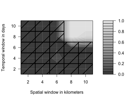
mwa in R using
citation(package = 'mwa')