Multifear is an R package designed to perform multiverse analyses for human conditioning data.
You can install via CRAN with the following command:
install.packages("multifear")For the development version, you can use the following command:
# Install devtools package in case it is not yet installed
install.packages("devtools")
devtools::install_github("AngelosPsy/multifear")
The package can be loaded with the following code:
library(multifear)We will start with a basic example of how the package works. This example includes a single group. After that, we will see how we can run the same analyses when we want to test between group effects.
First let’s load some additional packages that we need for our example.
suppressPackageStartupMessages(library(dplyr))
suppressPackageStartupMessages(library(ggplot2))
Now we will use some simulated data set that are included as example
data in the multifear package. In principle, you can use
any data including conditioned responses (e.g., skin conductance). You
can load the simulated data in your R environment as follows:
data("example_data")From these data we are going to select only the 10 first lines – it saves a lot of time for computation for this example. Here are the first 10 rows of the data set:
head(example_data, 10)
#>    id       CSP1       CSP2       CSP3      CSP4      CSP5      CSP6      CSP7
#> 1   2 0.62905570 0.92988220  1.0415000 0.9330014 0.9743682 0.8855119 0.8418664
#> 2   3 7.07953400 4.97656500 12.7791100 8.2847610 4.9798520 8.8685450 8.2468480
#> 3   4 0.00000000 1.21569500  2.4367400 4.5100300 5.3372170 4.6831920 3.6484020
#> 4   5 1.43786800 0.97055850  0.3784756 1.4434960 0.4060977 1.6015840 1.5274500
#> 5   7 0.94540620 3.29359400  3.4376340 2.7078930 3.6439630 3.8878390 3.6174920
#> 6   8 3.23735900 2.34393600  2.3931960 2.2908990 1.9583950 2.5094320 2.4234050
#> 7   9 0.43832140 0.04669674  0.2307273 2.2448410 1.6178050 1.8630760 1.7384420
#> 8  10 0.03912846 0.20814220  0.4654428 0.5395534 0.4498870 0.5519411 0.4144870
#> 9  11 0.88479390 1.64638700  0.9605724 0.7427042 0.2084812 2.2864430 1.8098150
#> 10 12 2.61601700 2.23660600  2.5479610 1.8130030 2.6899810 2.0758690 3.1323380
#>         CSP8      CSP9     CSP10       CSM1      CSM2      CSM3       CSM4
#> 1  0.9821523 0.5790559 0.3824215  0.9857365 1.2673990 0.0000000 0.64031250
#> 2  0.7607041 1.7655060 2.1758810 13.6548600 0.9066070 0.0000000 2.91306300
#> 3  2.1018580 6.4756940 2.6422620  0.0000000 3.2380020 2.4289650 0.25262940
#> 4  1.1900760 0.3994079 0.6168466  1.3146440 0.0000000 0.6570014 1.37108400
#> 5  2.2854040 5.2819210 4.5153330  4.2762160 3.1962110 3.4280200 1.88772700
#> 6  2.7189870 3.7545760 0.5508313  2.7552620 2.2843320 0.1147742 0.42298280
#> 7  1.5976320 0.8726718 2.5473010  0.3066088 1.5306480 2.1478420 0.46613780
#> 8  0.3175979 0.4557406 0.3433352  0.2956061 0.1793028 0.2681102 0.05366129
#> 9  1.7349280 1.8654570 0.9060298  1.2088490 0.4465152 0.8923611 1.56732600
#> 10 3.2265350 2.5452310 1.8400320  3.1200790 1.4983390 1.4273640 0.24111750
#>          CSM5       CSM6      CSM7       CSM8       CSM9      CSM10 group
#> 1  0.05137117 0.03480838 0.0000000 0.00000000 0.29036070 0.31496240     1
#> 2  0.60658980 3.72999700 1.1069910 3.63702500 0.00000000 0.00000000     2
#> 3  0.00000000 2.51429900 0.0000000 0.18621060 0.52076760 0.95751230     1
#> 4  0.53106310 0.54313130 0.2875019 0.00000000 0.18795960 0.18725370     2
#> 5  3.06479700 2.91668000 2.7914400 1.22984300 3.37716300 2.70570100     1
#> 6  2.22446600 0.00000000 0.0000000 1.21598600 0.00000000 0.00000000     2
#> 7  0.16134580 0.91540300 0.0000000 0.30176180 0.08460228 0.09295772     1
#> 8  0.10903030 0.00000000 0.0000000 0.04329369 0.19495150 0.30379580     2
#> 9  0.02774107 0.39216860 0.1940482 1.33170800 0.41266960 0.00000000     1
#> 10 0.72851310 0.96242680 0.0000000 1.27084300 0.03120063 0.00000000     2
A bit of explanation of the column names. With the column name ‘id’ we denote the participant number. Columns that contain the conditioned responses for conditioned stimulus plus (CS+) are denoted with column names starting with ‘CSP’. The number next to this name (1, 2, …, 10) is the trial number. The same goes for columns starting with ‘CSM’ but these denote conditioned responses in CS- trials. At this point the package only supports a single CS+ and a single CS-. Also, the package assumes that trials are following each other – so trial 2 comes after trial 1 etc.
Let’s visualize the data (such visualizations are not available in
the package but they can be carried out easily using the
graphics or the ggplot2 packages):
datmelt <- example_data %>%
  select(-id) %>%
  colMeans() %>%
  reshape2::melt(dat) %>%
  mutate(variable = rownames(.)) %>%
  mutate(cs = stringr::str_sub(variable, 1, 3),
  time = stringr::str_sub(variable, 4, 5))

  ggplot(data = datmelt, aes(x = time, y = value, group = cs)) +
  geom_line(aes(linetype = cs)) +
  geom_point(aes(shape = cs))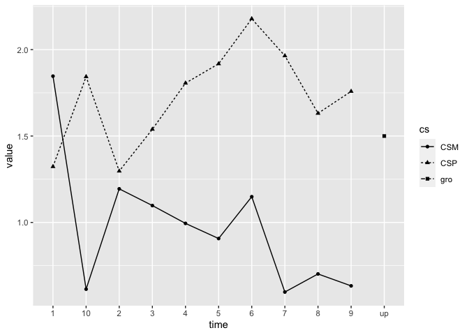
We see the basic learning pattern where CS+ responses end up being higher than CS- responses.
Now we need to analyse the data. For this we will use the multifear::universe_cs function. In order for this function to work, we need to provide the following arguments.
CS1: This will be the column names that contain the conditioned responses for the CS+ (i.e., CSP1 until CSP10).
CS2: This will be the column names that contain the conditioned response for the CS- (i.e., CSM1 until CSM10).
data: This is our data frame that contain that data for the CS+, CS-, as well as the column with the participant number.
group. In case of a group, then we need to specify the column with the group name. The default option is that there are no groups. In this first example we do not use any groups but we will do that in our second example – see below.
phase. Here we define the conditioning phase that the data were collected in (e.g., acquisition phase, extinction phase, etc). Please note that in case the user has multiple phases, she/he needs to run the function separately for each phases.
There are some other options in the function, such as defining the type of conditioning response. However, these are not necessary for now. So, let’s now run the function:
cs1 <- paste0("CSP", 1:10)
cs2 <- paste0("CSM", 1:10)
example_data <- example_data[1:10, ]
res <- multifear::universe_cs(cs1 = cs1, cs2 = cs2, data = example_data,
                              subj = "id", group = NULL, phase = "acquisition", include_bayes = FALSE)
And here are the results:
res
#> # A tibble: 4 × 20
#>   x       y     exclusion cut_off   model    controls method p.value effect.size
#>   <chr>   <chr> <chr>     <chr>     <chr>    <lgl>    <chr>    <dbl>       <dbl>
#> 1 cs      scr   full data full data t-test   NA       great… 0.00244      0.577
#> 2 cs      scr   full data full data t-test   NA       two.s… 0.00488      0.577
#> 3 cs:time scr   full data full data rep ANO… NA       rep A… 0.0152       0.0296
#> 4 cs      scr   full data full data rep ANO… NA       rep A… 0.00488      0.147
#> # ℹ 11 more variables: effect.size.lci <dbl>, effect.size.hci <dbl>,
#> #   effect.size.ma <dbl>, effect.size.ma.lci <dbl>, effect.size.ma.hci <dbl>,
#> #   estimate <dbl>, statistic <dbl>, conf.low <dbl>, conf.high <dbl>,
#> #   framework <chr>, data_used <list>
Let’s go through each column separately
x : is the effect that you are testing. For example, the cs means that you are testing cs differences. cs:time the cs X time interaction is tested. Be careful: when testing interactions, we only report the highest order interaction. That means that if you have a cs x time interaction, you do not get the results of the cs or the time main effect.
y: the dependent variable. In the example this is the scr responses.
exclusion: This columns reports as to what data were included in the data set. For example, here you see that we have only full data sets – no exclusion. This is because the multifear::universe_cs() only analyses full data sets. If we want to apply some exclusion criteria, we need to run the multifear::multiverse_cs() function – see later on.
model: What model was used. For example, here we see t-tests, and rep ANOVA (which means repeated measures ANOVA).
controls: This column is left empty. I included it because the specs R package had it so we may need to use it later on.
method: The method is a combination of the model and x column. Not really necessary if the other two columns exist.
p.value: The p-value of the test
estimate: The estimate that is returned from the test. Keep in mind though that this applies only for the t-test at the moment. We need to see what we can do for the ANOVA,
statistic. The statistic of the test
conf.low and conf.high In case you have an estimate, this returns the low and high levels of it
framework were the data analysed within a NHST or Bayesian framework?
data_used Here you have a data frame with the data used for the performed analyses. This is because someone maybe wants to recreate the results and also as a check that nothing went wrong.
Now, we want to perform the same analyses but for different data reduction procedures (see below). We can do it simply by:
res_multi <- multifear::multiverse_cs(cs1 = cs1, cs2 = cs2, data = example_data,
                                      subj = "id", group = NULL,
                                      phase = "acquisition",
                                      include_bayes = TRUE, include_mixed = TRUE)
#> Skipping ANOVA due to the number of trials for the cs1 and/or cs2.
res_multi
#> # A tibble: 116 × 21
#>    x         y     exclusion cut_off model controls method   p.value effect.size
#>    <chr>     <chr> <chr>     <chr>   <chr> <lgl>    <chr>      <dbl>       <dbl>
#>  1 cs        scr   full_data full d… t-te… NA       great…  2.44e- 3      0.577
#>  2 cs        scr   full_data full d… t-te… NA       two.s…  4.88e- 3      0.577
#>  3 cs        scr   full_data full d… Baye… NA       Bayes… NA            NA
#>  4 cs        scr   full_data full d… Baye… NA       Bayes… NA            NA
#>  5 cs:time   scr   full_data full d… rep … NA       rep A…  1.52e- 2      0.0296
#>  6 cs        scr   full_data full d… rep … NA       rep A…  4.88e- 3      0.147
#>  7 cscs2     scr   full_data <NA>    mixe… NA       mixed…  1.80e-13     NA
#>  8 cscs2:ti… scr   full_data <NA>    mixe… NA       mixed…  5.92e- 7     NA
#>  9 cscs2     scr   full_data <NA>    mixe… NA       mixed…  1.82e- 5     NA
#> 10 cscs2:ti… scr   full_data <NA>    mixe… NA       mixed…  2.16e- 2     NA
#> # ℹ 106 more rows
#> # ℹ 12 more variables: effect.size.lci <dbl>, effect.size.hci <dbl>,
#> #   effect.size.ma <dbl>, effect.size.ma.lci <dbl>, effect.size.ma.hci <dbl>,
#> #   estimate <dbl>, statistic <dbl>, conf.low <dbl>, conf.high <dbl>,
#> #   framework <chr>, data_used <list>, efffect.size.ma <lgl>
In terms of calling the function, we see that we need exactly the
same arguments as before. Internally, the function actually applies the
multifear::universe_cs but now apart from the full data
set, also for the data sets with different data inclusion procedures.
Whether each line refers to the full data set or any of the exclusion
criteria, we can see on the column exclusion criteria or in the
data_used column, although there it is difficult to see what happened
and it serves only reproduction criteria. So, the easiest thing to do is
to see the exclusion column. Now, it has the following levels:
res_multi$exclusion %>% unique()
#> [1] "full_data"  "ten_per"    "min_first"  "th3_per"    "halves"
#> [6] "fltrials"   "twenty_per" "fl2trials"  "per2trials"
The explanation of each level is the following:
fl2trials: first and last two trials.
fltrials: first and last trial
full_data: full data set
halves: use the first and last half of the trial. So, if you have 10 trials, you will have the first 5 and last 5 trials
min_first: take all trials apart from the first one
separate trials per 2
separate trials per 10%
separate trials per 33%
separate trials per 20%
This is the most challenging part. For now you can use the following function and you will get:
A histogram will all the p value and a red line showing the significance limit – by default alpha = 0.05
A histogram will all the Bayes factors and a red line showing the limit of inconclusive evidence – by default this is 0
Mean and median p values
the number of p values below the significance level
Mean and median of Bayes factors
the proportion of Bayes factors above 1
multifear::inference_cs(res_multi, na.rm = TRUE)
#>   mean_p_value median_p_value sd_p_value prop_p_value mean_bf_value
#> 1    0.1074323     0.00638261  0.2341194     82.35294       1855.05
#>   median_bf_value sd_bf_value prop_bf_value
#> 1        1.403218    9970.071      52.94118
And here we have a barplot of the results:
multifear::inference_plot(res_multi, add_line = FALSE)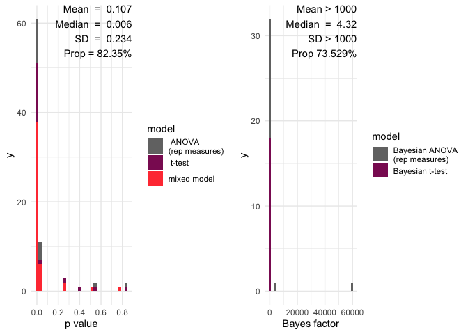
#> TableGrob (1 x 2) "arrange": 2 grobs
#>   z     cells    name           grob
#> 1 1 (1-1,1-1) arrange gtable[layout]
#> 2 2 (1-1,2-2) arrange gtable[layout]
Lastly, to plot the effect sizes, you can use the following function for the within-subjects effects:
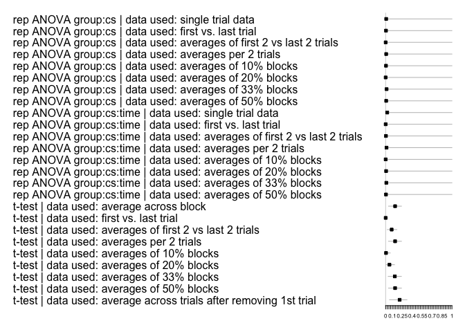
multifear::forestplot_mf(res_multi)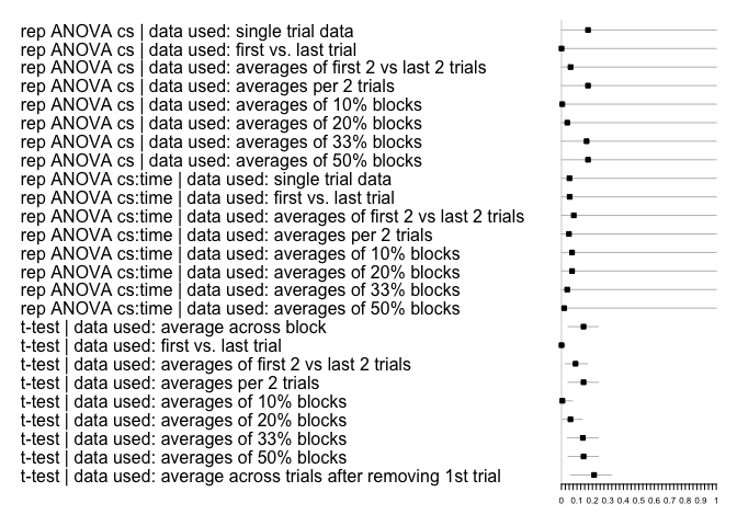
Importantly, multifear is able to run the same analyses
as in example 1 even when groups are included. This can be simply done
by defining the name of the column that includes the group levels (in
the example data set that name is “group” but you can use any other
name). Then, you can just run the same line of code as in example 1,
after defying the group parameter, as follows:
res_multi_group <- multifear::multiverse_cs(cs1 = cs1, cs2 = cs2,
                                            data = example_data, subj = "id",
                                            group = "group", phase = "acquisition",
                                            include_bayes = TRUE, include_mixed = TRUE)
#> Skipping ANOVA due to the number of trials for the cs1 and/or cs2.
res_multi_group
#> # A tibble: 116 × 21
#>    x         y     exclusion cut_off model controls method   p.value effect.size
#>    <chr>     <chr> <chr>     <chr>   <chr> <lgl>    <chr>      <dbl>       <dbl>
#>  1 cs        scr   full_data full d… t-te… NA       great…  2.44e- 3     0.577
#>  2 cs        scr   full_data full d… t-te… NA       two.s…  4.88e- 3     0.577
#>  3 cs        scr   full_data full d… Baye… NA       Bayes… NA           NA
#>  4 cs        scr   full_data full d… Baye… NA       Bayes… NA           NA
#>  5 group:cs… scr   full_data full d… rep … NA       rep A…  3.43e- 1     0.00288
#>  6 group:cs  scr   full_data full d… rep … NA       rep A…  4.60e- 1     0
#>  7 cscs2     scr   full_data <NA>    mixe… NA       mixed…  1.80e-13    NA
#>  8 cscs2:ti… scr   full_data <NA>    mixe… NA       mixed…  5.92e- 7    NA
#>  9 cscs2     scr   full_data <NA>    mixe… NA       mixed…  1.82e- 5    NA
#> 10 cscs2:ti… scr   full_data <NA>    mixe… NA       mixed…  2.16e- 2    NA
#> # ℹ 106 more rows
#> # ℹ 12 more variables: effect.size.lci <dbl>, effect.size.hci <dbl>,
#> #   effect.size.ma <dbl>, effect.size.ma.lci <dbl>, effect.size.ma.hci <dbl>,
#> #   estimate <dbl>, statistic <dbl>, conf.low <dbl>, conf.high <dbl>,
#> #   framework <chr>, data_used <list>, efffect.size.ma <lgl>
Accordingly, the inference plots look as follows:
multifear::inference_plot(res_multi_group, add_line = FALSE)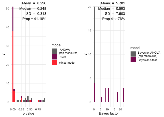
#> TableGrob (1 x 2) "arrange": 2 grobs
#>   z     cells    name           grob
#> 1 1 (1-1,1-1) arrange gtable[layout]
#> 2 2 (1-1,2-2) arrange gtable[layout]
Lastly, here are the forestoplot for the second example:
multifear::forestplot_mf(res_multi_group)