
![]()
The goal of mshap is to allow SHAP values for two-part models to be easily computed. A two-part model is one where the output from one model is multiplied by the output from another model. These are often used in the Actuarial industry, but have other use cases as well.
This package is designed in R with the example use cases
having models and shap values calculated in python. It is the hope that
the interoperability between the two languages continues to grow, and
the example here makes a strong case for the ease of transitioning
between the two.
Install mSHAP from CRAN with the following code:
install.packages("mshap")Or the development version from github with:
# install.packages("devtools")
devtools::install_github("srmatth/mshap")We will demonstrate a simple use case on simulated data. Suppose that we wish to be able to predict to total amount of money a consumer will spend on a subscription to a software product. We might simulate 4 explanatory variables that looks like the following:
## R
set.seed(16)
age <- runif(1000, 18, 60)
income <- runif(1000, 50000, 150000)
married <- as.numeric(runif(1000, 0, 1) > 0.5)
sex <- as.numeric(runif(1000, 0, 1) > 0.5)
# For the sake of simplicity we will have these as numeric already, where 0 represents male and 1 represents female
Now because this is a contrived example, we will knowingly set the
response variables as follows (suppose here that
cost_per_month is usage based, so as to be continuous):
## R
cost_per_month <- (0.0006 * income - 0.2 * sex + 0.5 * married - 0.001 * age) + 10
num_months <- 15 * (0.001 * income  * 0.001 * sex * 0.5 * married - 0.05 * age)^2
Thus, we have our data. We will combine the covariates into a single data frame for ease of use in python.
## R
X <- data.frame(age, income, married, sex)
The end goal of this exercise is to predict the total revenue from
the given customer, which mathematically will be
cost_per_month * num_months. Instead of multiplying these
two vectors together initially, we will instead create two models: one
to predict cost_per_month and the other to predict
num_months. We can then multiply the output of the two
models together to get our predictions.
We now move over to python to create our two models and predict on the training sets:
## Python
X = r.X
y1 = r.cost_per_month
y2 = r.num_months

cpm_mod = sk.RandomForestRegressor(n_estimators = 100, max_depth = 10, max_features = 2)
cpm_mod.fit(X, y1)
#> RandomForestRegressor(max_depth=10, max_features=2)
nm_mod = sk.RandomForestRegressor(n_estimators = 100, max_depth = 10, max_features = 2)
nm_mod.fit(X, y2)
#> RandomForestRegressor(max_depth=10, max_features=2)
cpm_preds = cpm_mod.predict(X)
nm_preds = nm_mod.predict(X)

tot_rev = cpm_preds * nm_preds
We will now proceed to use TreeSHAP and subsequently mSHAP to explain the ultimate model predictions.
## Python

# because these are tree-based models, shap.Explainer uses TreeSHAP to calculate
# fast, exact SHAP values for each model individually
cpm_ex = shap.Explainer(cpm_mod)
cpm_shap = cpm_ex.shap_values(X)
cpm_expected_value = cpm_ex.expected_value

nm_ex = shap.Explainer(nm_mod)
nm_shap = nm_ex.shap_values(X)
nm_expected_value = nm_ex.expected_value
## R
final_shap <- mshap(
shap_1 = py$cpm_shap,
shap_2 = py$nm_shap,
ex_1 = py$cpm_expected_value,
ex_2 = py$nm_expected_value
)
head(final_shap$shap_vals)
#> # A tibble: 6 x 4
#> V1 V2 V3 V4
#> <dbl> <dbl> <dbl> <dbl>
#> 1 1149. -1200. 13.9 -11.8
#> 2 -2711. 1149. 5.69 -11.2
#> 3 -1027. 1301. 5.81 9.58
#> 4 -2064. -879. -0.916 -22.7
#> 5 3803. 2096. 37.7 -27.4
#> 6 -2146. 897. 25.4 -14.3
final_shap$expected_value
#> [1] 4398.19As a check, you can see that the expected value for mSHAP is indeed the expected value of the model across the training data.
## R
mean(py$tot_rev)
#> [1] 4398.19
We now have calculated the mSHAP values for the multiplied model outputs! This will allow us to explain our final model.
The mSHAP package comes with additional functions that can be used to
visualize SHAP values in R. What is show here are the default outputs,
but these functions return {ggplot2} objects that are
easily customizable.
## R
summary_plot(
  variable_values = X,
  shap_values = final_shap$shap_vals,
  names = c("age", "income", "married", "sex") # this is optional, since X has column names
)
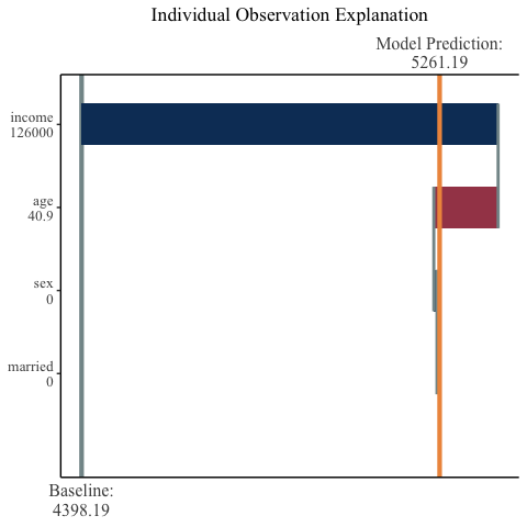
## R
observation_plot(
  variable_values = X[23,],
  shap_values = final_shap$shap_vals[23,],
  expected_value = final_shap$expected_value,
  names = c("age", "income", "married", "sex")
)
For another, more complex, use case run
vignette("mshap"). For more examples and options for
plotting, run vignette("mshap_plots").
{mshap}, please cite mSHAP: SHAP Values for
Two-Part Models