![]()
![]()
The mmand R package provides tools for performing
mathematical morphology operations, such as erosion and dilation, or
finding connected components, on arrays of arbitrary dimensionality. It
can also smooth and resample arrays, obtaining values between pixel
centres or scaling the image up or down wholesale.
All of these operations are underpinned by three powerful functions,
which perform different types of kernel-based operations:
morph(), components() and
resample().
An additional function provides a multidimensional distance transform operation.
A test image of a jet engine fan is available within the package, and will be used for demonstration below. It can be read in and displayed using the code
library(mmand)
library(loder)

fan <- readPng(system.file("images", "fan.png", package="mmand"))
display(fan)
Here we are using the loder package to read the PNG file.
Mathematical
morphology is an image processing technique that can be used to
emphasise or remove certain types of features from binary or greyscale
images. It is classically performed on two-dimensional images, but can
be useful in three or more dimensions, as, for example, in medical image
analysis. The mmand package can work on R arrays of any
dimensionality, including one-dimensional vectors.
The basic operations in mathematical morphology are erosion and dilation. A simple one-dimensional example serves to illustrate their effects:
x <- c(0,0,1,0,0,0,1,1,1,0,0)
k <- c(1,1,1)
erode(x,k)
##  [1] 0 0 0 0 0 0 0 1 0 0 0
dilate(x,k)
##  [1] 0 1 1 1 0 1 1 1 1 1 0
The erode() function “thins out” areas in the input
vector, x, which were “on” (i.e. set to 1), to the point
where the first of these areas “disappears” entirely. Conversely, the
dilate() function expands these regions into neighbouring
pixels.
The vector k here is called the kernel or
structuring element. It effectively controls the region of
influence of the operation when it is applied to each value.
Derived from these basic operations are the opening and closing functions. These apply both basic operations, using the same kernel, but in different orders: an opening is an erosion followed by a dilation, whereas a closing is a dilation followed by an opening.
opening(x,k)
##  [1] 0 0 0 0 0 0 1 1 1 0 0
closing(x,k)
##  [1] 0 0 1 0 0 0 1 1 1 0 0
Notice that, in this case, the closing gets us back to where we started, whereas the opening does not. This is because the initial erosion operation removes the first “on” block entirely, so it cannot be recovered by the subsequent dilation. Hence, the effect is to remove small features that are narrower than the kernel.
Mathematical morphology is not limited to binary data. When generalised to greyscale images, erosion replaces each nonzero pixel with the minimum value within the kernel when it is centred at that pixel, and dilation uses the maximum. For example,
x <- c(0,0,0.5,0,0,0,0.2,0.5,0.3,0,0)
erode(x,k)
##  [1] 0.0 0.0 0.0 0.0 0.0 0.0 0.0 0.2 0.0 0.0 0.0
Notice that the remaining nonzero value is now reduced from 0.5 to 0.2, the minimum value across the original pixel and its neighbours on either side. With a wider kernel, its final value would have dropped to zero.
The effect is more intuitively demonstrated on a real two-dimensional image:
k <- shapeKernel(c(3,3), type="diamond")
display(erode(fan, k))
Notice that darker areas appear enlarged. In this case the kernel is
itself a 2D array (or matrix), and unlike the 1D case there is a choice
of plausible shapes for a particular width. The
shapeKernel() function will create box, disc and diamond
shaped kernels, and their higher-dimensional equivalents.
Using a wider kernel exaggerates the effect:
k <- shapeKernel(c(7,7), type="diamond")
display(erode(fan, k))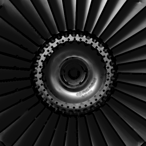
In the case above, the diamond shape of the kernel is obvious in areas where the kernel is larger than the eroded features.
Note that the kernel may also be anisotropic, i.e. it may have a different width in each dimension:
k <- shapeKernel(c(7,3), type="diamond")
display(erode(fan, k))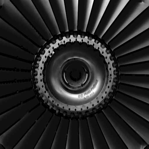
The effect of dilation is complementary, shrinking dark regions and enlarging bright ones:
k <- shapeKernel(c(3,3), type="diamond")
display(dilate(fan, k))
In this case the low-intensity and narrow handwriting towards the middle of the fan has all but disappeared.
The basic operations can be combined together for other useful purposes. For example, the difference between the dilated and eroded versions of an image, known as the morphological gradient, can be used to show up edges between areas of light and dark.
k <- shapeKernel(c(3,3), type="diamond")
display(dilate(fan,k) - erode(fan,k))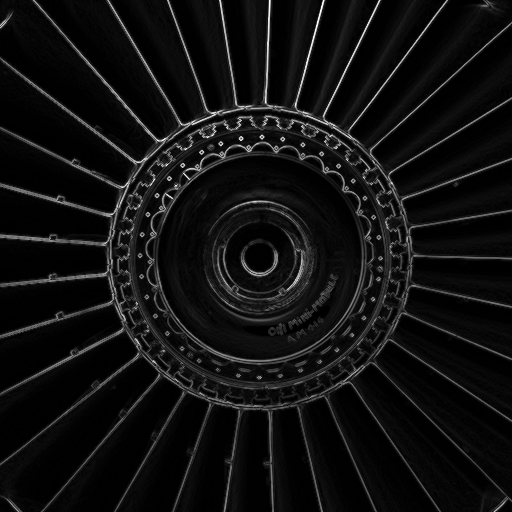
The Sobel filter has a similar effect.
display(sobelFilter(fan))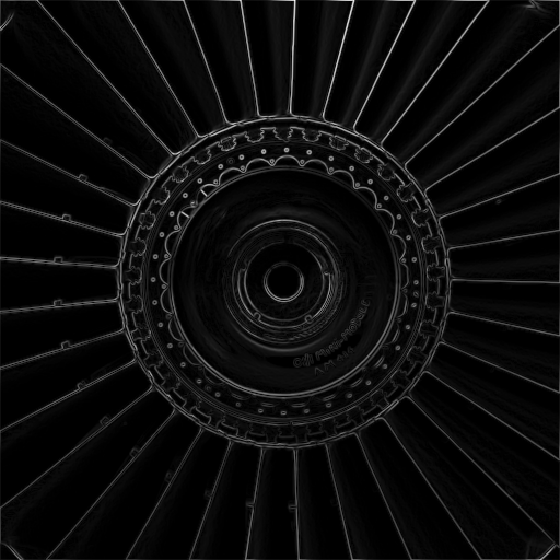
Topological skeletonisation is the process of thinning a shape to a medial line or surface representing the approximate path of the original. It can be thought of as the result of repeated erosion, up to the point where only a “core” of the shape exists. It is usually applied to binary data.
As of version 1.5.0, the mmand package offers three
different skeletonisation algorithms, with different advantages and
limitations. (Please see the documentation at ?skeletonise
for details.) Below we see the results of applying each of them in turn
to the outline of a capital letter B.
library(loder)
B <- readPng(system.file("images", "B.png", package="mmand"))
k <- shapeKernel(c(3,3), type="diamond")

display(B)
display(skeletonise(B,k,method="lantuejoul"), col="red", add=TRUE)
The B is shown alone first, and then with the three skeletons overlaid in red. (Only the code for generating the first is shown.) Notice that all three skeletons are reasonable medial paths, but the centre one (using Beucher’s formula) is a little thicker than the others in most places, and only the right one (using the hit-or-miss transform) is fully self-connected.
A loosely related operation is kernel-based smoothing, often used to ameliorate noise. In this case the kernel is used as a set of coefficients, which are multiplied by data within the neighbourhood of each pixel and added together. For these purposes the kernel should usually be normalised, so that its values add up to one.
Gaussian smoothing is a typical example, wherein our coefficients are
given by the probability densities of a Gaussian distribution centred at
the middle of the kernel. The mmand package provides the
gaussianSmooth() function for performing this operation.
Below we can see an example in one dimension, where we create some noisy
data and then approximately recover the underlying cosine function by
applying smoothing.
x <- seq(0, 4*pi, pi/64)
y <- cos(x) + runif(length(x),-0.2,0.2)
y_smoothed <- gaussianSmooth(y, 6)

plot(x, y, pch=19, col="grey50", xaxt="n")
axis(1, (0:4)*pi, expression(0,pi,2*pi,3*pi,4*pi))
lines(x, y_smoothed, lwd=2)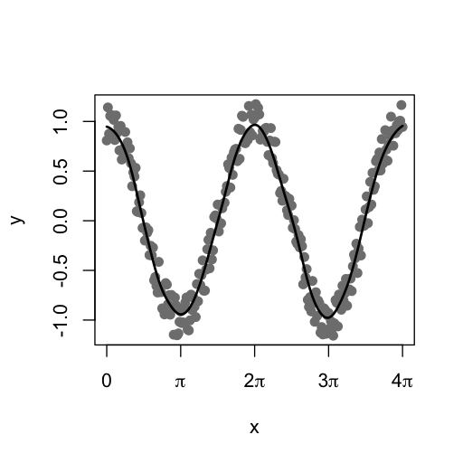
It should be borne in mind that the second argument to the
gaussianSmooth() function is the standard
deviation of the smoothing Gaussian kernel in each dimension,
rather than the kernel size.
On our two-dimensional test image, which contains no appreciable noise, the effect is to blur the picture. Indeed, this operation is sometimes called Gaussian blurring.
display(gaussianSmooth(fan, c(3,3)))
An alternative approach to noise reduction is median filtering,
and mmand provides another function for this purpose:
k <- shapeKernel(c(3,3), type="box")
display(medianFilter(fan, k))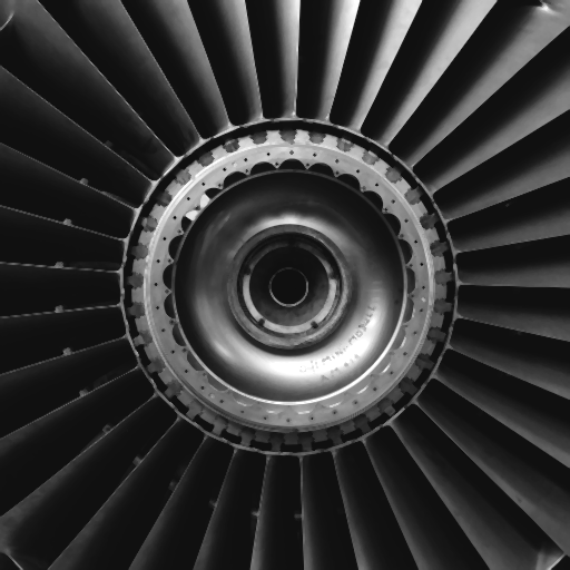
This method is typically better at preserving edges in the image, which can be desirable in some applications.
Every operation described so far has been based on
mmand’s flexible morph() function, which uses
a kernel represented by an array to select pixels of interest in
morphing the image, optionally using the kernel’s elements to adjust
their values, and then applying a merge operation of some sort (sum,
minimum, maximum, median, etc.) to produce the pixel value in the final
image. In every case the result has the same size as the original data
array.
In the next section we will examine operations that change the array’s dimensions, but first we consider another useful operation: finding connected components. This is the task of assigning a label to each contiguous subregion of an array.
To demonstrate, we start by first thresholding the fan image using
k-means clustering (with k=2). The package’s
threshold() function can be used for this:
fan_thresholded <- threshold(fan, method="kmeans")
display(fan_thresholded)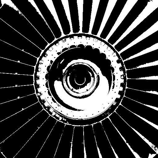
We can then find the connected components. In this case the kernel determines which pixels are deemed to be neighbours. For example,
k <- shapeKernel(c(3,3), type="box")
fan_components <- components(fan_thresholded, k)
Now we can visualise the result by assigning a colour to each component.
display(fan_components, col=rainbow(max(fan_components,na.rm=TRUE)))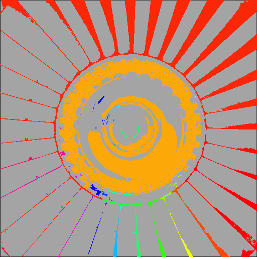
As we might expect, the largest components—which label only the “on” areas of the image—correspond to (most of) the ring of fan blades, and the bright part of the central hub.
This is can be a useful tool for “segmentation”, or dividing an image into coherent areas.
A useful operation in certain contexts is the distance transform, which calculates the distance from each pixel to a region of interest. There are signed an unsigned variants, with the former also calculating the distance to the boundary within the region of interest itself. We can use the thresholded image from above to illustrate the point:
display(distanceTransform(fan_thresholded))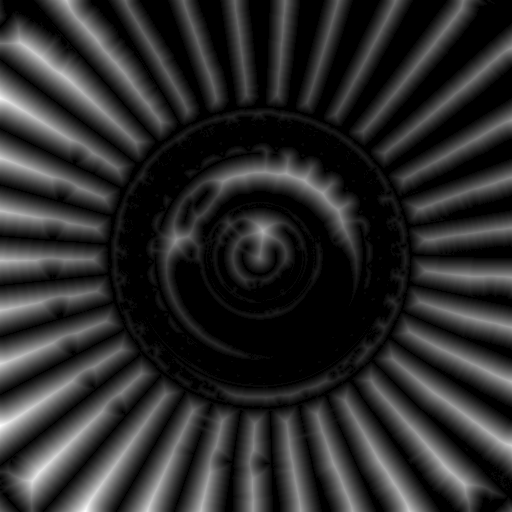
display(abs(distanceTransform(fan_thresholded, signed=TRUE)))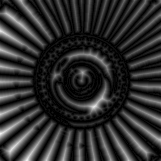
We take the absolute value of the signed transform here for ease of visual interpretation. Notice how, in both cases, bright “ridges” in the transformed image correspond to midlines at maximal distance from the boundary between foreground and background. Philip Rideout provides a detailed explanation of the algorithm and its uses.
The final category of problems that mmand can solve uses
a different type of kernel to resample an image at arbitrary points, or
on a new grid. This allows images to be resized, or arrays to be indexed
using non-integer indices. The kernels in these cases are functions,
which provide coefficients for using data at any distance from the new
pixel location to determine its value.
Let’s use an example to illustrate this. Consider the simple vector
x <- c(0,0,1,0,0)Its second element is 0, and its third element is 1, but what is its value at index 2.5? One answer is that it simply doesn’t have one, but if these were samples from a fundamentally continuous source, then there is conceptually a value everywhere. We just didn’t capture it. Our best guess would have to be that it is either 0 or 1, or something in between. If we try to use 2.5 as an index we get the value 0:
x[2.5]
## [1] 0
(R simply truncates 2.5 to 2 and returns element 2.) The
resample() function provides a set of alternatives:
resample(x, 2.5, triangleKernel())
## [1] 0.5
Now we obtain the value 0.5, which does not appear anywhere in the
original, but it is the average of the values at locations 2 and 3. In
this case, therefore, resample() is performing linear
interpolation.
The triangle kernel is just one possible function for interpolating
the data. Another option is the box kernel, generated by
boxKernel(), which simply returns the “nearest” value in
the original data. Yet another option is provided by
mitchellNetravaliKernel(), or mnKernel() for
short, which provides a family of cubic spline kernels proposed by
Mitchell and Netravali (DOI: 10.1145/378456.378514). We can see the
profile of any of these kernels by plotting them:
plot(mitchellNetravaliKernel(1/3, 1/3))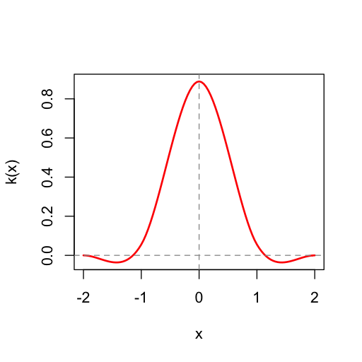
In higher dimensions, the resampled point locations can be passed to
resample() either as a matrix giving the points to sample
at, one per row, or as a list giving the locations on each axis, which
will be made into a grid.
A common use for resampling is to scale an image up or down. The
rescale() function is a convenience wrapper around
resample() for scaling an array by a given scale factor.
Here, we can use it to scale a smaller version of the fan image up to
the size of the larger version:
library(loder)

fan_small <- readPng(system.file("images", "fan-small.png", package="mmand"))
dim(fan_small)
## [1] 128 128   1

display(rescale(drop(fan_small), 4, mnKernel()))
The scaled-up image of course has less detail than the original 512x512 pixel version, since it is based on 16 times fewer data points, but the general features of the fan are perfectly discernible.