![]()
![]()
![]()
![]()
The goal of metaconfoundr is to make it easy to visualize confounding control in meta-analyses. Researchers use a causal diagram to assess factors that are required to control for to estimate an effect unbiased by confounding. Then, the researchers create a data frame of confounding variables and how well each study in the meta-analysis controlled for each: adequately, inadequately, or with some control. See the vignette on collecting confounder data for more information.
In addition to the package, metaconfoundr ships with a Shiny app to
help create visualizations. You can start the app locally with
launch_metaconfoundr_app() or use the hosted
version.
Install the most recent released version of metaconfoundr from CRAN:
install.packages("metaconfoundr")You can install the development version of metaconfoundr from GitHub with:
# if needed
# install.packages("remotes")
remotes::install_github("malcolmbarrett/metaconfoundr")metaconfoundr includes an example dataset, ipi, that
contains information on a meta-analysis of interpregnancy interval and
the risk of preterm birth. Use metaconfoundr() to prepare
the dataset to work with metaconfoundr functions. ipi
includes several domains of confounders, but for ease of visualization,
we will just show one, Sociodemographics.
library(metaconfoundr)
mc_ipi <- metaconfoundr(ipi) %>%
  dplyr::filter(construct == "Sociodemographics")

mc_ipi
#> # A tibble: 55 × 5
#>    construct         variable     is_confounder study        control_quality
#>    <chr>             <chr>        <chr>         <chr>        <ord>
#>  1 Sociodemographics Maternal age Y             Zhu_2001a    adequate
#>  2 Sociodemographics Maternal age Y             Zhu_2001b    adequate
#>  3 Sociodemographics Maternal age Y             Zhu_1999     adequate
#>  4 Sociodemographics Maternal age Y             Smith_2003   adequate
#>  5 Sociodemographics Maternal age Y             Shachar_2016 adequate
#>  6 Sociodemographics Maternal age Y             Salihu_2012a adequate
#>  7 Sociodemographics Maternal age Y             Salihu_2012b adequate
#>  8 Sociodemographics Maternal age Y             Hanley_2017  adequate
#>  9 Sociodemographics Maternal age Y             deWeger_2011 adequate
#> 10 Sociodemographics Maternal age Y             Coo_2017     adequate
#> # … with 45 more rows
metaconfoundr includes several tools for visualizing the results of a
confounding control assesment. The most common are
mc_heatmap() and mc_trafficlight().
mc_heatmap(mc_ipi)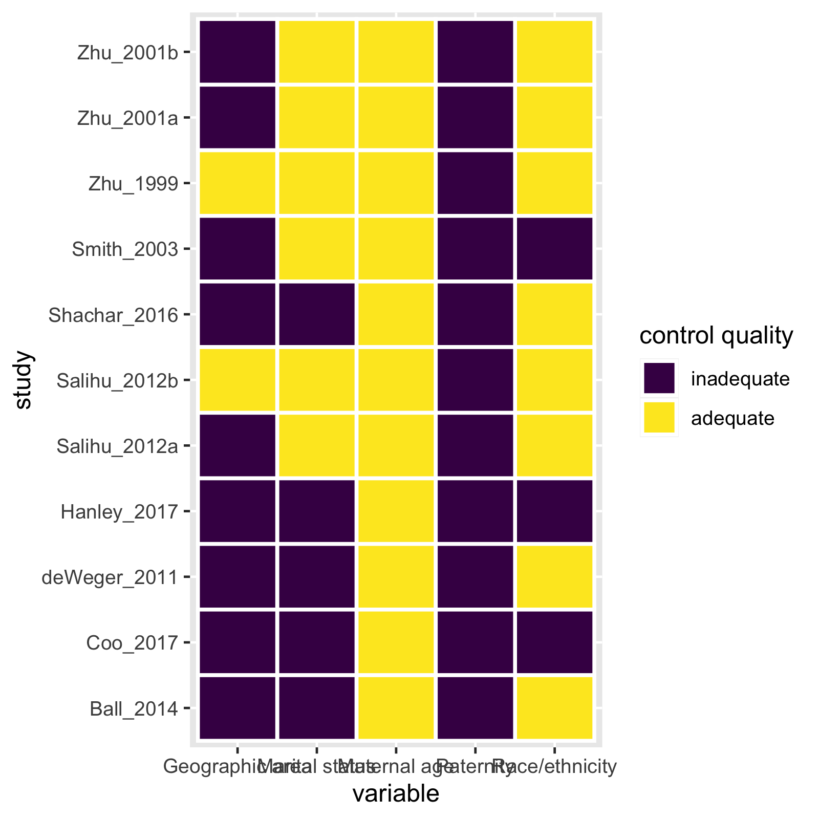
mc_trafficlight(mc_ipi)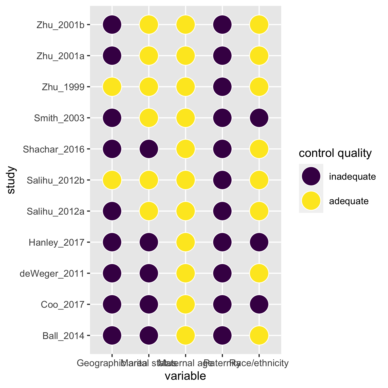
These plotting functions return ggplots, so they are easy to modify.
mc_heatmap(mc_ipi) +
  theme_mc() +
  ggplot2::guides(x = ggplot2::guide_axis(n.dodge = 2))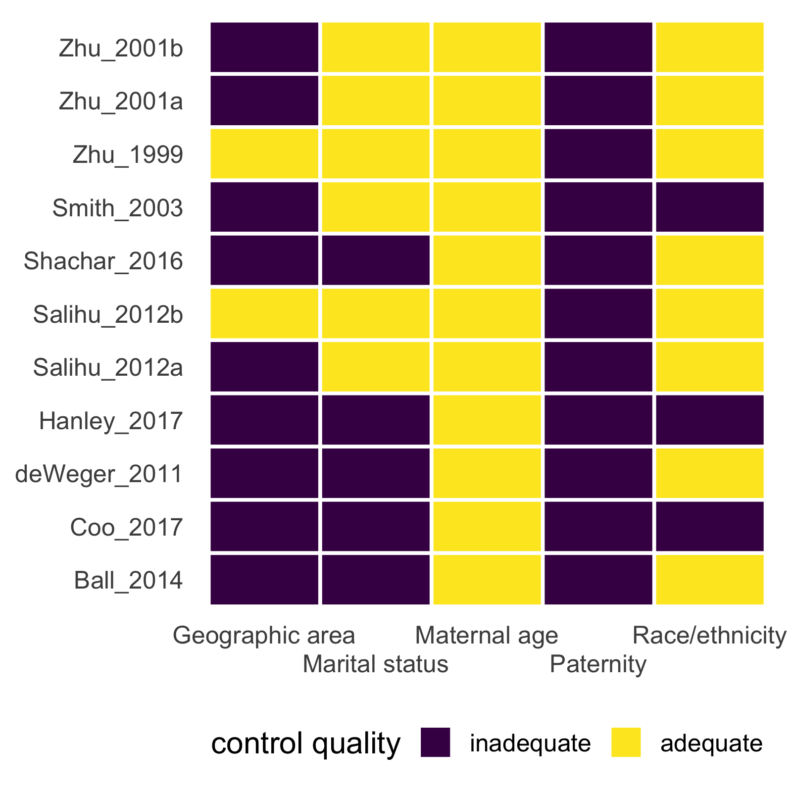
metaconfoundr also includes geoms and scales to make output similar to other types of bias assessments for meta-analyses.
mc_trafficlight(mc_ipi) +
  theme_mc() +
  geom_cochrane() +
  scale_fill_cochrane()  +
  ggplot2::guides(x = ggplot2::guide_axis(n.dodge = 2))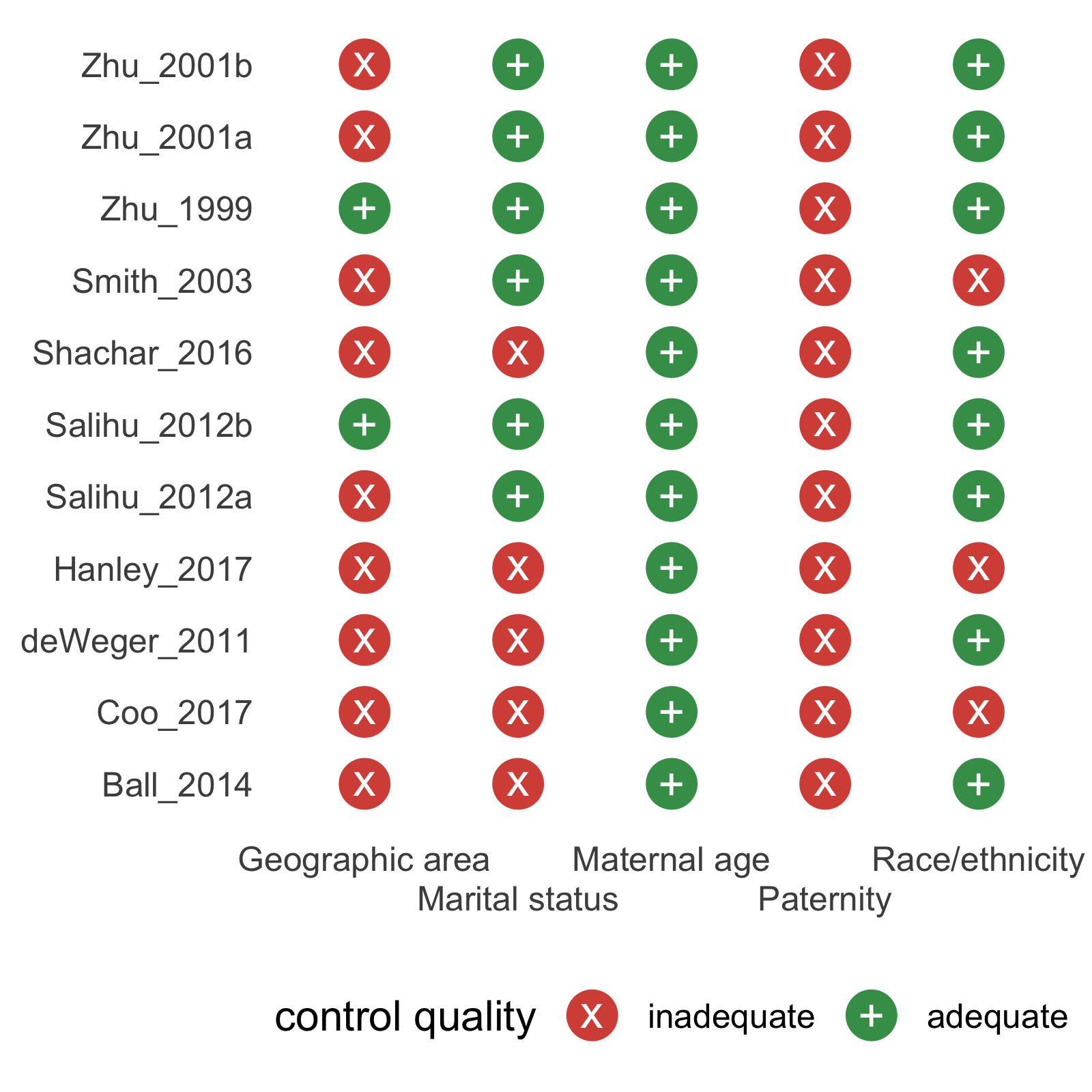
For working with common assessments of bias in studies, such as the ROBINS tool, see the excellent robvis package.
Please note that the metaconfoundr project is released with a Contributor Code of Conduct. By contributing to this project, you agree to abide by its terms.