mcStats

================ This package is used to visualize distributions in relation to traditional hypothesis tests. We have found that students are capable of interpreting p-values, but often struggle with understanding how they relate to the underlying distribution. The stats package performs statistical tests while we visualize the results.

Hypothesis Tests

Proportion Test

showProp.Test(3, 10)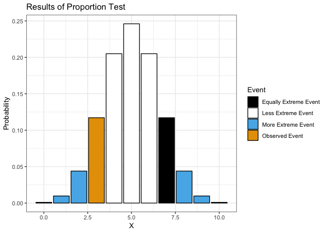

## 
##  Exact binomial test
## 
## data:  x and n
## number of successes = 3, number of trials = 10, p-value = 0.3438
## alternative hypothesis: true probability of success is not equal to 0.5
## 95 percent confidence interval:
##  0.06673951 0.65245285
## sample estimates:
## probability of success 
##                    0.3

T-Test

One Sample

Test with null hypothesis mean = 0.

x <- rnorm(10)
showT.Test(x)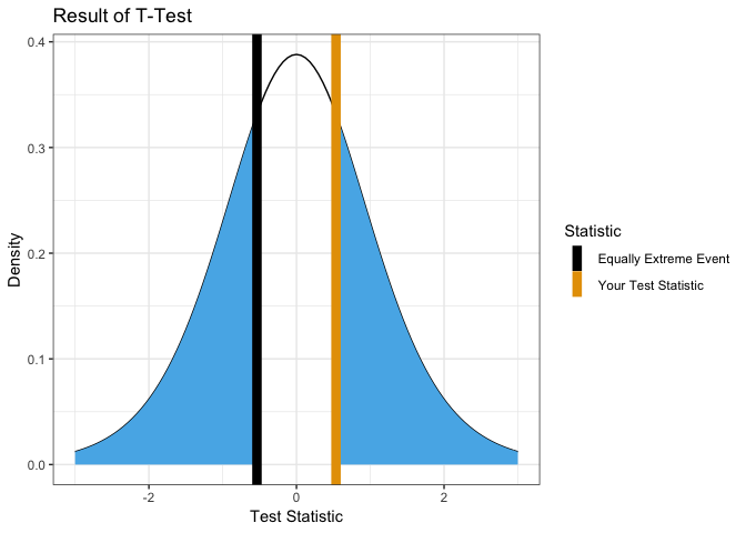

## 
##  One Sample t-test
## 
## data:  group1
## t = -0.97931, df = 9, p-value = 0.353
## alternative hypothesis: true mean is not equal to 0
## 95 percent confidence interval:
##  -0.9367283  0.3707214
## sample estimates:
##  mean of x 
## -0.2830035

Test with null hypothesis mean = 0.5.

showT.Test(x, mu = 0.5)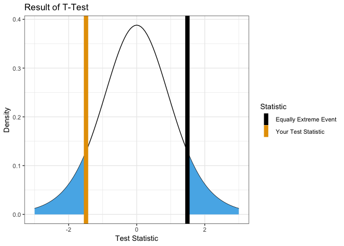

## 
##  One Sample t-test
## 
## data:  group1
## t = -2.7095, df = 9, p-value = 0.02402
## alternative hypothesis: true mean is not equal to 0.5
## 95 percent confidence interval:
##  -0.9367283  0.3707214
## sample estimates:
##  mean of x 
## -0.2830035

Two Sample

y <- rnorm(10, mean = 0.1)
showT.Test(x,y)

Chi-Square Test

Mosaic Plot

x <- matrix(runif(9,5,100), ncol = 3, dimnames = list(c("Yes1", "No1", "Maybe 1"),
                                                      c("Yes2", "No2", "Maybe 2")))
mosaicplot(x)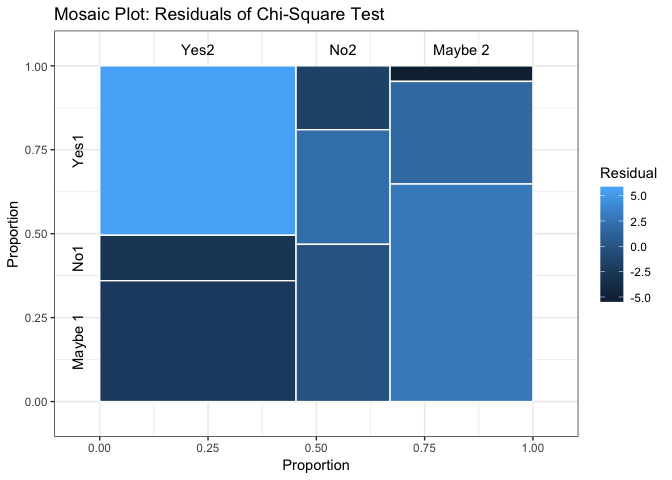

Distribution

showChiSq.Test(x)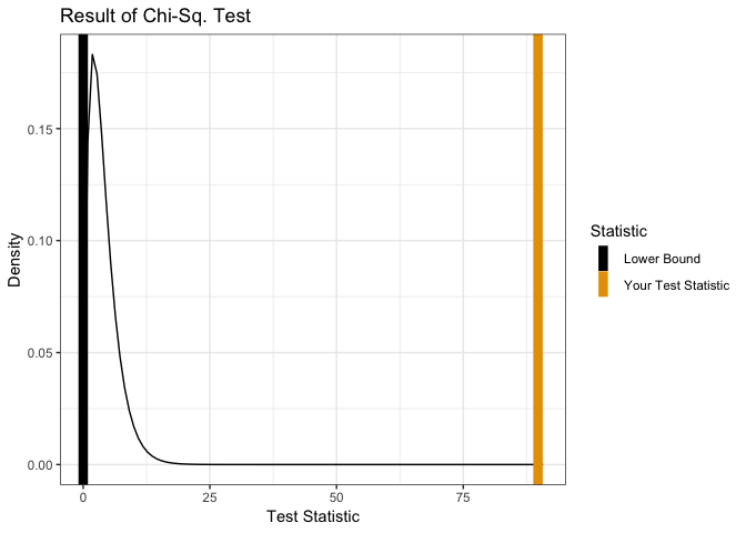

## 
##  Pearson's Chi-squared test
## 
## data:  x
## X-squared = 20.445, df = 4, p-value = 0.0004078

McNemar Test

Performance <-
  matrix(c(794, 86, 150, 570),
         nrow = 2,
         dimnames = list("1st Survey" = c("Approve", "Disapprove"),
                         "2nd Survey" = c("Approve", "Disapprove")))
showMcNemarTest(Performance)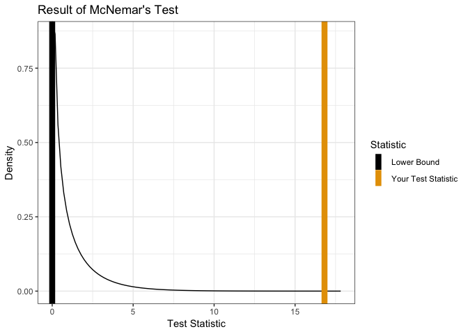

## 
##  McNemar's Chi-squared test with continuity correction
## 
## data:  x
## McNemar's chi-squared = 16.818, df = 1, p-value = 4.115e-05

Bootstrap

bootstrap(mean, x, 0, 100)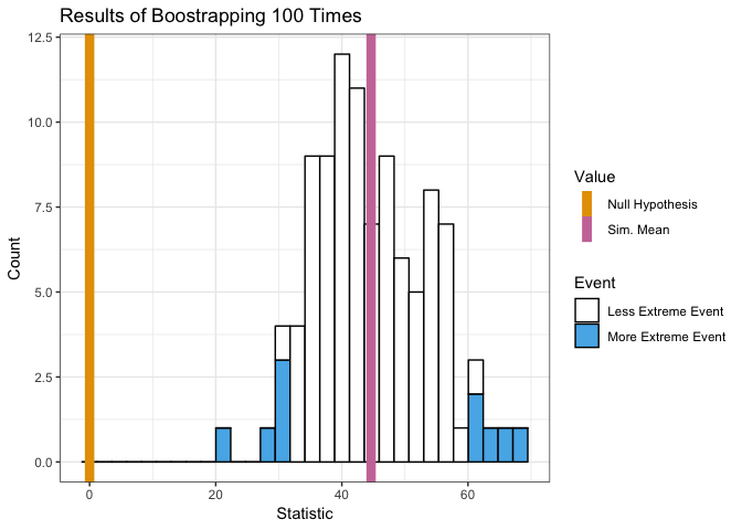

##   [1] 54.90774 51.07035 62.03353 59.45124 42.65071 53.54602 58.19805
##   [8] 49.23022 42.80682 48.37725 55.93226 43.66260 38.76233 37.54761
##  [15] 48.67384 42.42315 64.43235 68.48759 55.88688 54.98819 45.01146
##  [22] 44.32679 44.94303 52.94193 40.54650 47.56330 46.70979 42.63162
##  [29] 34.53033 64.46052 42.53795 46.94533 41.18465 36.09311 48.51360
##  [36] 50.08601 58.49279 44.25783 47.79896 45.98412 63.10048 50.72895
##  [43] 62.70815 70.40356 44.79826 44.72806 55.45402 44.30009 48.20786
##  [50] 42.41185 59.92486 43.56006 43.01403 32.92129 49.30569 36.82319
##  [57] 46.08493 51.61663 51.93606 58.78356 26.15019 69.00779 59.82237
##  [64] 49.10645 56.87518 50.13957 49.68720 33.95228 51.20886 44.01459
##  [71] 66.88024 38.29459 63.04476 45.01572 56.02155 61.85452 56.19405
##  [78] 55.77186 49.30737 43.08087 44.30009 37.41971 55.21450 41.24469
##  [85] 49.87103 68.78172 47.83253 50.72265 48.07421 52.72435 48.62027
##  [92] 40.54171 55.14868 51.01445 43.22471 50.76491 54.59131 50.19763
##  [99] 55.68494 57.43471

ANOVA

showANOVA(yield ~  N + P + K, npk)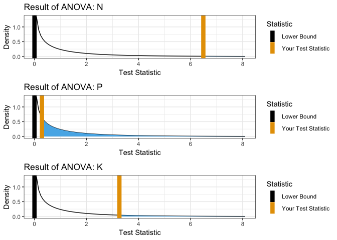

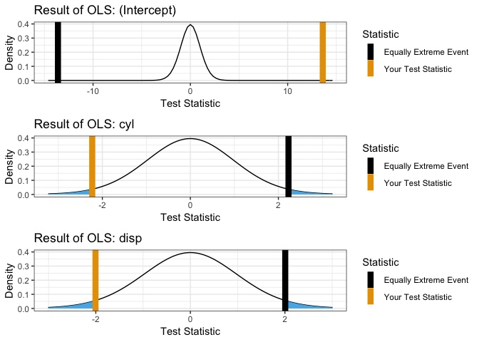
OLS

showOLS(mpg ~ cyl + disp, mtcars)