![]()
![]()
The markets package provides tools to estimate and analyze an equilibrium and four disequilibrium models. The equilibrium model can be estimated with either two-stage least squares or with full information maximum likelihood. The two methods are asymptotically equivalent. The disequilibrium models are estimated using full information maximum likelihood. The likelihoods can be estimated both with independent and correlated demand and supply shocks. The optimization of the likelihoods can be performed either using analytic expressions or numerical approximations of their gradients. A detailed overview of the package’s functionality, usage examples, and design traits is given in Karapanagiotis (2024).
The five models of the package are described by systems of simultaneous equations, with the equilibrium system being the only linear one, while the disequilibrium systems being non-linear. All models specify the demand and the supply side of the market by a linear (in parameters) equation. The remaining equations of each model, if any, further specify the market structure.
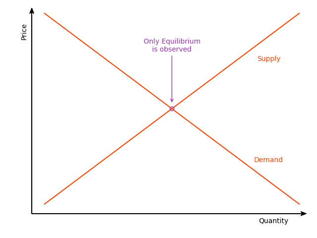
The equilibrium model adds the market-clearing condition to the demand and supply equations of the system. For the system to be identifiable, at least one variable on the demand side must not be present on the supply side and vice versa. This model assumes that the market observations always represent equilibrium points in which the demanded and supplied quantities are equal. The model can be estimated using two-stage least squares (Theil 1953) or full information maximum likelihood (Karapanagiotis, n.d.). Asymptotically, these methods are equivalent (Balestra and Varadharajan-Krishnakumar 1987).
\[
\left.
\begin{aligned}
D_{n t} &= X_{d, n t}'\beta_{d} + P_{n t}\alpha_{d} + u_{d, n t}
\\
S_{n t} &= X_{s, n t}'\beta_{s} + P_{n t}\alpha_{s} + u_{s, n t}
\\
Q_{n t} &= D_{n t} = S_{n t}
\end{aligned}
\right. \qquad\text{(EM)}
\]
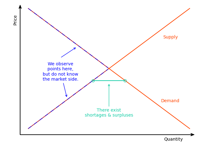
The basic model is the simplest disequilibrium model of the package as it basically imposes no assumption on the market structure regarding price movements (Fair and Jaffee 1972; Maddala and Nelson 1974). In contrast with the equilibrium model, the market-clearing condition is replaced by the short-side rule, which stipulates that the minimum between the demanded and supplied quantities is observed. The econometrician does not need to specify whether an observation belongs to the demand or the supply side since the estimation of the model will allocate the observations on the demand or supply side so that the likelihood is maximized.
\[
\left.
\begin{aligned}
D_{n t} &= X_{d, n t}'\beta_{d} + u_{d, n t} \\
S_{n t} &= X_{s, n t}'\beta_{s} + u_{s, n t} \\
Q_{n t} &= \min\{D_{n t},S_{n t}\}
\end{aligned}
\right. \qquad\text{(BM)}
\]
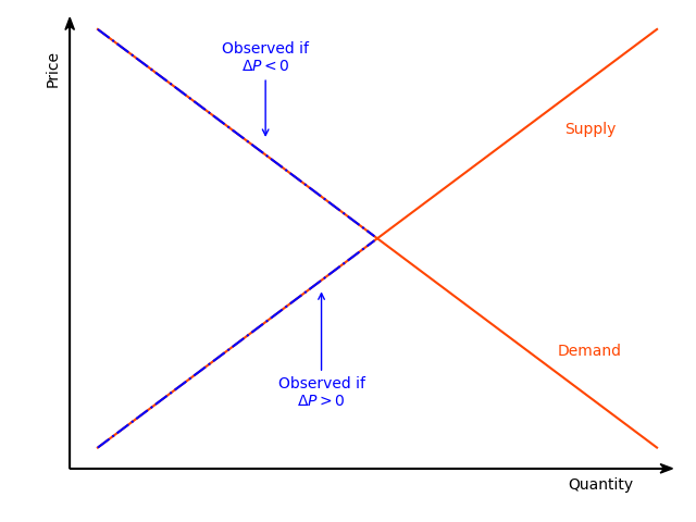
The directional model attaches an additional equation to the system of the basic model. The added equation is a sample separation condition based on the direction of the price movements (Fair and Jaffee 1972; Maddala and Nelson 1974). When prices increase at a given date, an observation is assumed to belong on the supply side. When prices fall, an observation is assumed to belong on the demand side. In short, this condition separates the sample before the estimation and uses this separation as additional information in the estimation procedure. Although, when appropriate, more information improves estimations, it also, when inaccurate, intensifies misspecification problems. Therefore, the additional structure of the directional model does not guarantee better estimates in comparison with the basic model.
\[
\left.
\begin{aligned}
D_{n t} &= X_{d, n t}'\beta_{d} + u_{d, n t} \\
S_{n t} &= X_{s, n t}'\beta_{s} + u_{s, n t} \\
Q_{n t} &= \min\{D_{n t},S_{n t}\} \\
\Delta P_{n t} &\ge 0 \implies D_{n t} \ge S_{n t}
\end{aligned}
\right. \qquad\text{(DM)}
\]
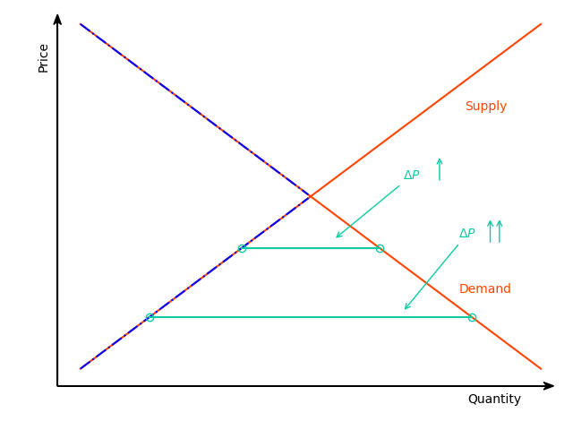
The separation rule of the directional model classifies observations on the demand- or supply-side based in a binary fashion, which is not always flexible, as observations that correspond to large shortages/surpluses are treated the same as observations that correspond to small shortages/ surpluses. The deterministic adjustment model of the package replaces this binary separation rule with a quantitative one (Fair and Jaffee 1972; Maddala and Nelson 1974). The magnitude of the price movements is analogous to the magnitude of deviations from the market-clearing condition. This model offers a flexible estimation alternative, with one extra degree of freedom in the estimation of price dynamics, that accounts for market forces that are in alignment with standard economic reasoning. By letting \(\gamma\) approach zero, the equilibrium model can be obtained as a limiting case of this model.
\[
\left.
\begin{aligned}
D_{n t} &= X_{d, n t}'\beta_{d} + P_{n t}\alpha_{d} + u_{d, n t}
\\
S_{n t} &= X_{s, n t}'\beta_{s} + P_{n t}\alpha_{s} + u_{s, n t}
\\
Q_{n t} &= \min\{D_{n t},S_{n t}\} \\
\Delta P_{n t} &= \frac{1}{\gamma} \left( D_{n t} - S_{n t} \right)
\end{aligned}
\right. \qquad\text{(DA)}
\]
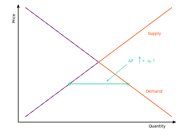
The last model of the package extends the price dynamics of the deterministic adjustment model by adding additional explanatory variables and a stochastic term. The latter term, in particular, makes the price adjustment mechanism stochastic and, deviating from the structural assumptions of models \((DA)\) and \((DM)\), abstains from imposing any separation assumption on the sample (Maddala and Nelson 1974; Quandt and Ramsey 1978). The estimation of this model offers the highest degree of freedom, accompanied, however, by a significant increase in estimation complexity, which can hinder the stability of the procedure and the numerical accuracy of the outcomes.
\[
\left.
\begin{aligned}
D_{n t} &= X_{d, n t}'\beta_{d} + P_{n t}\alpha_{d} + u_{d, n t}
\\
S_{n t} &= X_{s, n t}'\beta_{s} + P_{n t}\alpha_{s} + u_{s, n t}
\\
Q_{n t} &= \min\{D_{n t},S_{n t}\} \\
\Delta P_{n t} &= \frac{1}{\gamma} \left( D_{n t} - S_{n t} \right)
+ X_{p, n t}'\beta_{p} + u_{p, n t}
\end{aligned}
\right. \qquad\text{(SA)}
\]
The released version of markets can be installed from CRAN with:
install.packages("markets")The source code of the in-development version can be downloaded from GitHub.
After installing it, there is a basic-usage example installed with it. To see it type the command
vignette('basic_usage')Online documentation is available for both the released and in-development versions
of the package. The documentation files can also be accessed in
R by typing
?? marketsThis is a basic example that illustrates how a model of the package can be estimated. The package is loaded in the standard way.
library(markets)The example uses simulated data. The markets package offers a function to simulate data from data-generating processes that correspond to the models that the package provides.
model_tbl <- simulate_data(
  "diseq_basic", 10000, 5,
  -1.9, 36.9, c(2.1, -0.7), c(3.5, 6.25),
  2.8, 34.2, c(0.65), c(1.15, 4.2),
  NA, NA, c(NA),
  seed = 42
)
Models are initialized by a constructor. In this example, a basic disequilibrium model is estimated. There are also other models available (see Design and functionality). The constructor sets the model’s parameters and performs the necessary initialization processes. The following variables specify this example’s parameterization.
The models can be estimated both with panel and time series data.
The constructor expects both a subject and a time identifier in order to
perform the necessary initialization operations (these are respectively
given by id and date in the simulated data of
this example). The observation identification of the data is
automatically generated by composing the subject and time identifiers.
The resulting composite key is the combination of columns that uniquely
identify a record of the dataset.
The observable traded quantity variable (given by Q
in this example’s simulated data). The demanded and supplied quantities
are not observable, and they are identified either based on the market
clearing condition or the short-side rule.
The price variable, which is named after P in the
simulated data.
The right-hand side specifications of the demand and supply equations. The expressions are specified similarly to the expressions of formulas of linear models. Indicator variables and interactions are created automatically by the constructor.
The verbosity level controls the level of messaging. The object displays
verbose <- 0correlated_shocks <- TRUEThe model is estimated with default options by a simple call. See the
documentation of estimate for more details and options.
fit <- diseq_basic(
  Q | P | id | date ~ P + Xd1 + Xd2 + X1 + X2 | P + Xs1 + X1 + X2,
  model_tbl, correlated_shocks = correlated_shocks, verbose = verbose
)
The results can be inspected in the usual fashion via
summary.
summary(fit)## Basic Model for Markets in Disequilibrium:
## Demand RHS : D_P + D_Xd1 + D_Xd2 + D_X1 + D_X2
## Supply RHS : S_P + S_Xs1 + S_X1 + S_X2
## Short Side Rule : Q = min(D_Q, S_Q)
## Shocks : Correlated
## Nobs : 50000
## Sample Separation : Not Separated
## Quantity Var : Q
## Price Var : P
## Key Var(s) : id, date
## Time Var : date
##
## Maximum likelihood estimation:
## Method : BFGS
## Convergence Status : success
## Starting Values :
## D_P D_CONST D_Xd1 D_Xd2 D_X1 D_X2 S_P
## 1.2430 32.8102 0.6986 -0.2362 1.9377 4.8826 1.2390
## S_CONST S_Xs1 S_X1 S_X2 D_VARIANCE S_VARIANCE RHO
## 32.8104 0.4500 1.9376 4.8819 3.8528 4.2008 0.0000
##
## Coefficients:
## Estimate Std. Error z value Pr(>|z|)
## D_P -1.924717799 0.013835435 -139.1150898 0.0000000 ***
## D_CONST 36.937193226 0.021936141 1683.8510012 0.0000000 ***
## D_Xd1 2.110785687 0.009406163 224.4045458 0.0000000 ***
## D_Xd2 -0.691555109 0.008147975 -84.8744788 0.0000000 ***
## D_X1 3.521398292 0.009739125 361.5723353 0.0000000 ***
## D_X2 6.262824545 0.009398391 666.3719793 0.0000000 ***
## S_P 2.797103009 0.007373930 379.3232361 0.0000000 ***
## S_CONST 34.188334232 0.007529995 4540.2861998 0.0000000 ***
## S_Xs1 0.663960433 0.005615403 118.2391348 0.0000000 ***
## S_X1 1.139702284 0.006086385 187.2543982 0.0000000 ***
## S_X2 4.203214203 0.005977236 703.2036046 0.0000000 ***
## D_VARIANCE 0.996663485 0.012531211 79.5344912 0.0000000 ***
## S_VARIANCE 1.006627503 0.008313621 121.0817230 0.0000000 ***
## RHO -0.009218528 0.026590170 -0.3466893 0.7288247
## ---
## Signif. codes: 0 '***' 0.001 '**' 0.01 '*' 0.05 '.' 0.1 ' ' 1
##
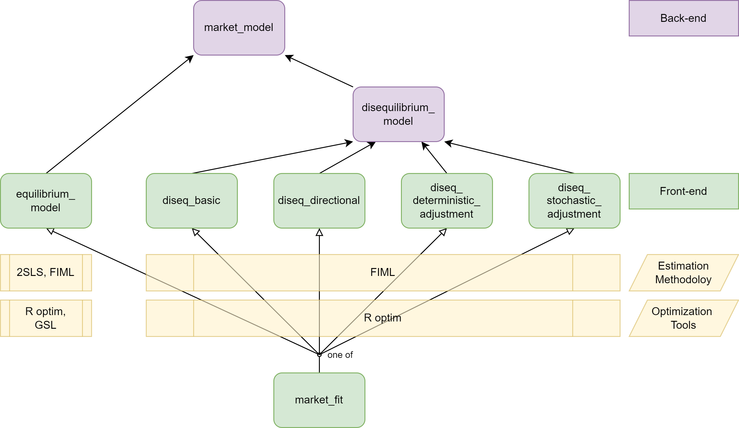
## -2 log L: 138460The equilibrium model can be estimated either using two-stage least squares or full information maximum likelihood. The two methods are asymptotically equivalent. The class for which both of these estimation methods are implemented is
equilibrium_model.In total, there are four disequilibrium models, which are all estimated using full information maximum likelihood. By default, the estimations use analytically calculated gradient expressions, but the user can override this behavior. The classes that implement the four disequilibrium models are
diseq_basic,diseq_directional,diseq_deterministic_adjustment, anddiseq_stochastic_adjustment.The package organizes these classes in a simple object-oriented hierarchy.
Concerning post-estimation analysis, the package offers functionality to calculate
The estimation of the basic model is also supported by the package Disequilibrium. By default, the Disequilibrium package numerically approximates the gradient when optimizing the likelihood. In contrast, markets uses analytically calculated expressions for the likelihood, which can reduce the duration of estimating the model. In addition, it allows the user to override this behavior and use the numerically approximated gradient. There is no alternative package that supports the out-of-the-box estimation of the other three disequilibrium models of markets.
The package is planned to be expanded in the following ways:
Feel free to join, share, contribute, and distribute.
The code is distributed under the MIT License.