


lavaan![]()
![]()
![]()
Affords an alternative, vector-based syntax to lavaan,
as well as other convenience functions such as naming paths and defining
indirect links automatically. Also offers convenience formatting
optimized for a publication and script sharing workflow.
You can install the lavaanExtra package directly from
CRAN:
install.packages("lavaanExtra")Or the development version from the r-universe (note that there is a 24-hour delay with GitHub):
install.packages("lavaanExtra", repos = c(
  rempsyc = "https://rempsyc.r-universe.dev",
  CRAN = "https://cloud.r-project.org"))
Or from GitHub, for the very latest version:
# If not already installed, install package `remotes` with `install.packages("remotes")`
remotes::install_github("rempsyc/lavaanExtra")
To see all the available functions, use:
help(package = "lavaanExtra")Dependencies: Because lavaanExtra is a
package of convenience functions relying on several external packages,
it uses (inspired by the easystats
packages) a minimalist philosophy of only installing packages that you
need when you need them through rlang::check_installed().
Should you wish to specifically install all suggested dependencies at
once (you can view the full list by clicking on the CRAN badge on this
page), you can run the following (be warned that this may take a long
time, as some of the suggested packages are only used in the vignettes
or examples):
install.packages("lavaanExtra", dependencies = TRUE)lavaanExtra?paste0() with
appropriate item numbers instead of typing each one every time.# Load libraries
library(lavaan)
library(lavaanExtra)
# Define latent variables
latent <- list(
visual = c("x1", "x2", "x3"),
textual = c("x4", "x5", "x6"),
speed = c("x7", "x8", "x9")
)
# If you have many items, you can also use the `paste0` function:
x <- paste0("x", 1:9)
latent <- list(
visual = x[1:3],
textual = x[4:6],
speed = x[7:9]
)
# Write the model, and check it
cfa.model <- write_lavaan(latent = latent)
cat(cfa.model)
#> ##################################################
#> # [-----Latent variables (measurement model)-----]
#>
#> visual =~ x1 + x2 + x3
#> textual =~ x4 + x5 + x6
#> speed =~ x7 + x8 + x9
# Fit the model fit and plot with `lavaanExtra::cfa_fit_plot`
# to get the factor loadings visually (optionally as PDF)
fit.cfa <- cfa_fit_plot(cfa.model, HolzingerSwineford1939)
#> lavaan 0.6-19 ended normally after 35 iterations
#>
#> Estimator ML
#> Optimization method NLMINB
#> Number of model parameters 21
#>
#> Number of observations 301
#>
#> Model Test User Model:
#> Standard Scaled
#> Test Statistic 85.306 87.132
#> Degrees of freedom 24 24
#> P-value (Chi-square) 0.000 0.000
#> Scaling correction factor 0.979
#> Yuan-Bentler correction (Mplus variant)
#>
#> Model Test Baseline Model:
#>
#> Test statistic 918.852 880.082
#> Degrees of freedom 36 36
#> P-value 0.000 0.000
#> Scaling correction factor 1.044
#>
#> User Model versus Baseline Model:
#>
#> Comparative Fit Index (CFI) 0.931 0.925
#> Tucker-Lewis Index (TLI) 0.896 0.888
#>
#> Robust Comparative Fit Index (CFI) 0.930
#> Robust Tucker-Lewis Index (TLI) 0.895
#>
#> Loglikelihood and Information Criteria:
#>
#> Loglikelihood user model (H0) -3737.745 -3737.745
#> Scaling correction factor 1.133
#> for the MLR correction
#> Loglikelihood unrestricted model (H1) -3695.092 -3695.092
#> Scaling correction factor 1.051
#> for the MLR correction
#>
#> Akaike (AIC) 7517.490 7517.490
#> Bayesian (BIC) 7595.339 7595.339
#> Sample-size adjusted Bayesian (SABIC) 7528.739 7528.739
#>
#> Root Mean Square Error of Approximation:
#>
#> RMSEA 0.092 0.093
#> 90 Percent confidence interval - lower 0.071 0.073
#> 90 Percent confidence interval - upper 0.114 0.115
#> P-value H_0: RMSEA <= 0.050 0.001 0.001
#> P-value H_0: RMSEA >= 0.080 0.840 0.862
#>
#> Robust RMSEA 0.092
#> 90 Percent confidence interval - lower 0.072
#> 90 Percent confidence interval - upper 0.114
#> P-value H_0: Robust RMSEA <= 0.050 0.001
#> P-value H_0: Robust RMSEA >= 0.080 0.849
#>
#> Standardized Root Mean Square Residual:
#>
#> SRMR 0.065 0.065
#>
#> Parameter Estimates:
#>
#> Standard errors Sandwich
#> Information bread Observed
#> Observed information based on Hessian
#>
#> Latent Variables:
#> Estimate Std.Err z-value P(>|z|) Std.lv Std.all
#> visual =~
#> x1 1.000 0.900 0.772
#> x2 0.554 0.132 4.191 0.000 0.498 0.424
#> x3 0.729 0.141 5.170 0.000 0.656 0.581
#> textual =~
#> x4 1.000 0.990 0.852
#> x5 1.113 0.066 16.946 0.000 1.102 0.855
#> x6 0.926 0.061 15.089 0.000 0.917 0.838
#> speed =~
#> x7 1.000 0.619 0.570
#> x8 1.180 0.130 9.046 0.000 0.731 0.723
#> x9 1.082 0.266 4.060 0.000 0.670 0.665
#>
#> Covariances:
#> Estimate Std.Err z-value P(>|z|) Std.lv Std.all
#> visual ~~
#> textual 0.408 0.099 4.110 0.000 0.459 0.459
#> speed 0.262 0.060 4.366 0.000 0.471 0.471
#> textual ~~
#> speed 0.173 0.056 3.081 0.002 0.283 0.283
#>
#> Variances:
#> Estimate Std.Err z-value P(>|z|) Std.lv Std.all
#> .x1 0.549 0.156 3.509 0.000 0.549 0.404
#> .x2 1.134 0.112 10.135 0.000 1.134 0.821
#> .x3 0.844 0.100 8.419 0.000 0.844 0.662
#> .x4 0.371 0.050 7.382 0.000 0.371 0.275
#> .x5 0.446 0.057 7.870 0.000 0.446 0.269
#> .x6 0.356 0.047 7.658 0.000 0.356 0.298
#> .x7 0.799 0.097 8.222 0.000 0.799 0.676
#> .x8 0.488 0.120 4.080 0.000 0.488 0.477
#> .x9 0.566 0.119 4.768 0.000 0.566 0.558
#> visual 0.809 0.180 4.486 0.000 1.000 1.000
#> textual 0.979 0.121 8.075 0.000 1.000 1.000
#> speed 0.384 0.107 3.596 0.000 1.000 1.000
#>
#> R-Square:
#> Estimate
#> x1 0.596
#> x2 0.179
#> x3 0.338
#> x4 0.725
#> x5 0.731
#> x6 0.702
#> x7 0.324
#> x8 0.523
#> x9 0.442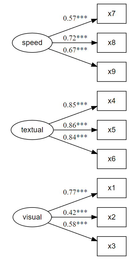
# Get nice fit indices with the `rempsyc::nice_table` integration
nice_fit(fit.cfa, nice_table = TRUE)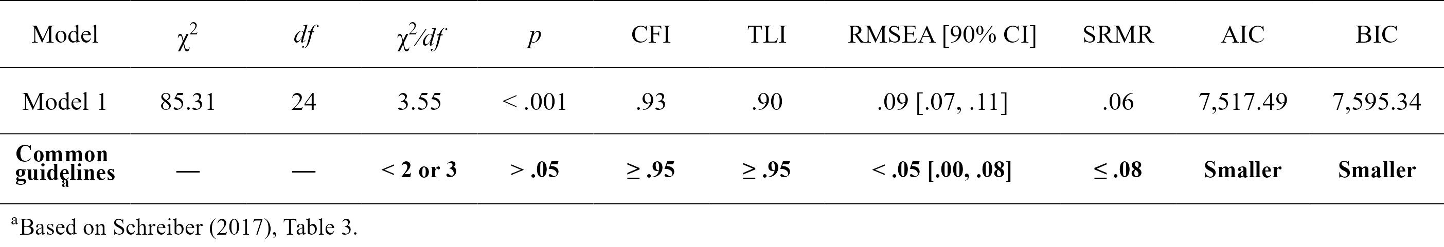
Note that latent variables have been defined above, so we can reuse them as is, without having to redefine them.
# Define our other variables
M <- "visual"
IV <- c("ageyr", "grade")
DV <- c("speed", "textual")

# Define our lavaan lists
mediation <- list(speed = M, textual = M, visual = IV)
regression <- list(speed = IV, textual = IV)
covariance <- list(speed = "textual", ageyr = "grade")

# Define indirect effects object
indirect <- list(IV = IV, M = M, DV = DV)

# Write the model, and check it
model <- write_lavaan(
  mediation = mediation,
  regression = regression,
  covariance = covariance,
  indirect = indirect,
  latent = latent,
  label = TRUE
)
cat(model)
#> ##################################################
#> # [-----Latent variables (measurement model)-----]
#>
#> visual =~ x1 + x2 + x3
#> textual =~ x4 + x5 + x6
#> speed =~ x7 + x8 + x9
#>
#> ##################################################
#> # [-----------Mediations (named paths)-----------]
#>
#> speed ~ visual_speed*visual
#> textual ~ visual_textual*visual
#> visual ~ ageyr_visual*ageyr + grade_visual*grade
#>
#> ##################################################
#> # [---------Regressions (Direct effects)---------]
#>
#> speed ~ ageyr + grade
#> textual ~ ageyr + grade
#>
#> ##################################################
#> # [------------------Covariances-----------------]
#>
#> speed ~~ textual
#> ageyr ~~ grade
#>
#> ##################################################
#> # [--------Mediations (indirect effects)---------]
#>
#> ageyr_visual_speed := ageyr_visual * visual_speed
#> ageyr_visual_textual := ageyr_visual * visual_textual
#> grade_visual_speed := grade_visual * visual_speed
#> grade_visual_textual := grade_visual * visual_textual

fit.sem <- sem(model, data = HolzingerSwineford1939)
# Get regression parameters and make pretty with `rempsyc::nice_table`
lavaan_reg(fit.sem, nice_table = TRUE, highlight = TRUE)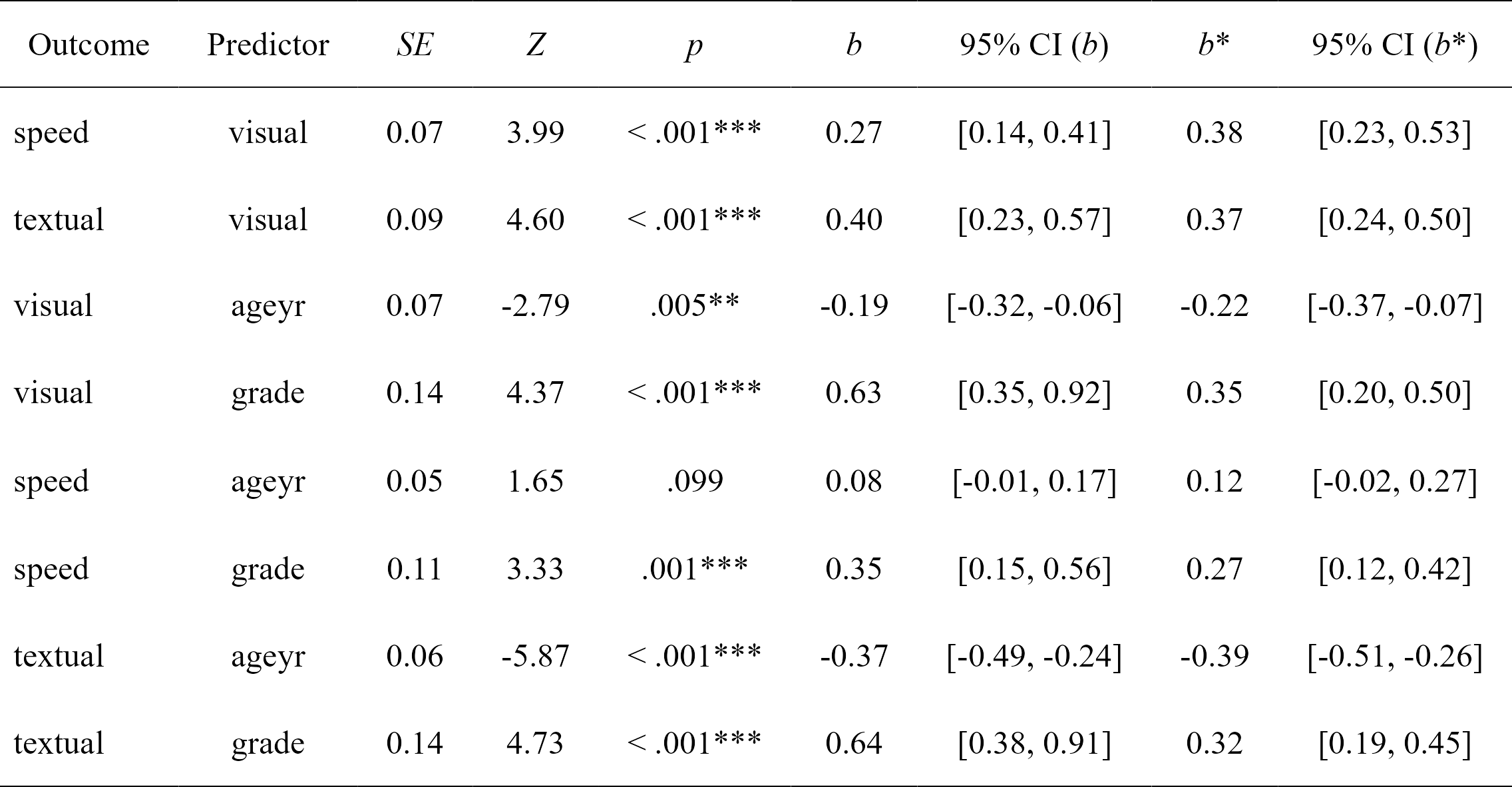
# Get covariances/correlations and make them pretty with
# the `rempsyc::nice_table` integration
lavaan_cor(fit.sem, nice_table = TRUE)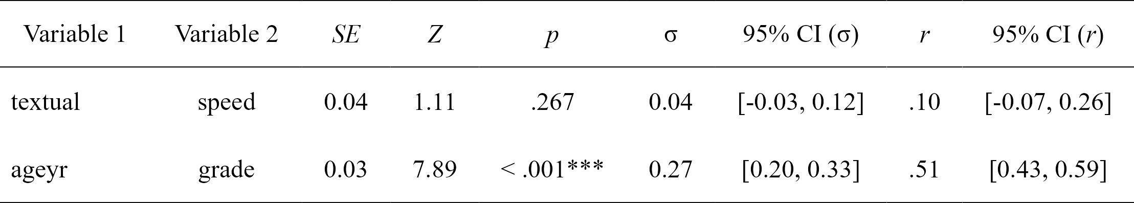
# Get nice fit indices with the `rempsyc::nice_table` integration
fit_table <- nice_fit(list(fit.cfa, fit.sem), nice_table = TRUE)
fit_table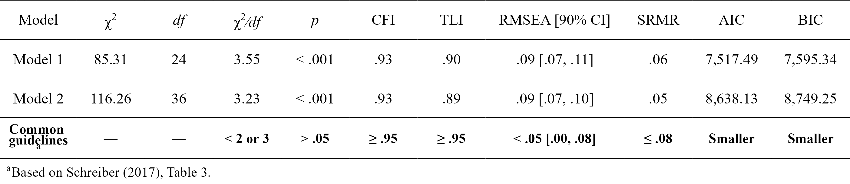
# Save fit table to Word!
flextable::save_as_docx(fit_table, path = "fit_table.docx")
# Note that it will also render to PDF in an `rmarkdown` document
# with `output: pdf_document`, but using `latex_engine: xelatex`
# is necessary when including Unicode symbols in tables like with
# the `nice_fit()` function.

# Let's get the user-defined (e.g., indirect) effects only and make it pretty
# with the `rempsyc::nice_table` integration
lavaan_defined(fit.sem, nice_table = TRUE)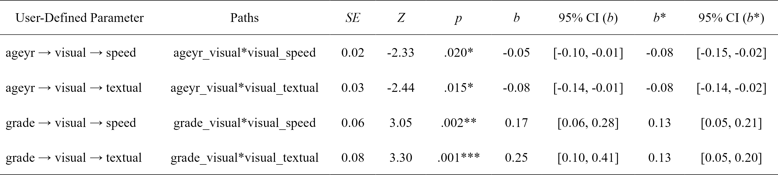
# Plot our model
nice_lavaanPlot(fit.sem)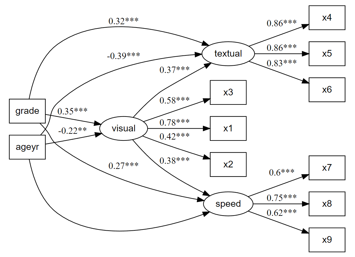
# Alternative way to plot
mylayout <- data.frame(
  IV = c("", "x1", "grade", "", "ageyr", "", ""),
  M = c("", "x2", "", "visual", "", "", ""),
  DV = c("", "x3", "textual", "", "speed", "", ""),
  DV.items = c(paste0("x", 4:6), "", paste0("x", 7:9))
) |>
  as.matrix()
mylayout
#>      IV      M        DV        DV.items
#> [1,] ""      ""       ""        "x4"
#> [2,] "x1"    "x2"     "x3"      "x5"
#> [3,] "grade" ""       "textual" "x6"
#> [4,] ""      "visual" ""        ""
#> [5,] "ageyr" ""       "speed"   "x7"
#> [6,] ""      ""       ""        "x8"
#> [7,] "" "" "" "x9"nice_tidySEM(fit.sem, layout = mylayout, label_location = 0.7)
ggplot2::ggsave("my_semPlot.pdf", width = 6, height = 6, limitsize = FALSE)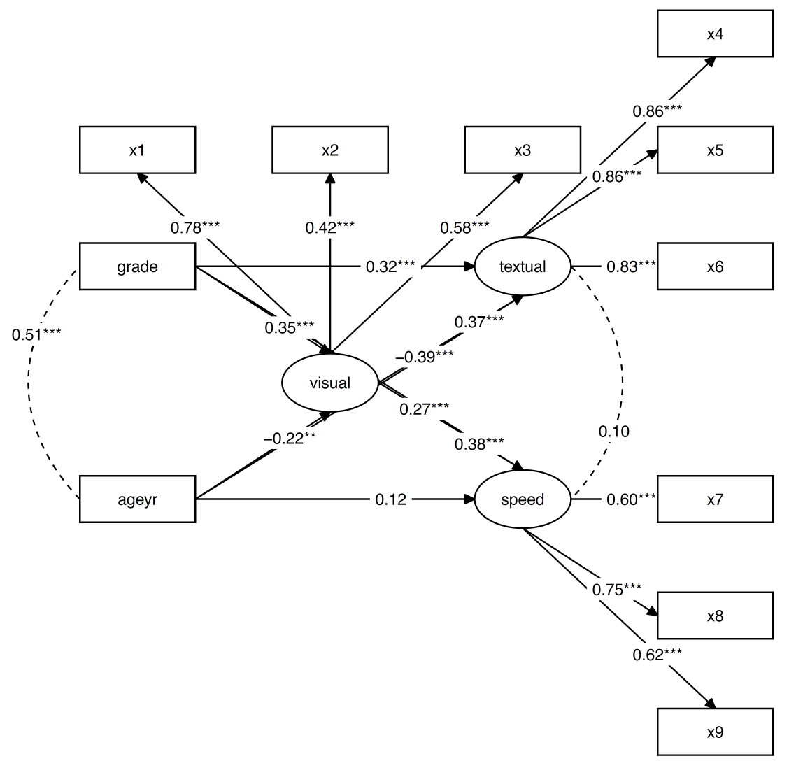
This is an experimental package in a very early stage. Any feedback or feature request is appreciated, and the package will likely change and evolve over time based on community feedback. Feel free to open an issue or discussion to share your questions or concerns. And of course, please have a look at the other tutorials to discover even more cool features: https://lavaanExtra.remi-theriault.com/articles/
Thank you for your support. You can support me and this package here: https://github.com/sponsors/rempsyc