![]()
![]()
Title: Higher-Level Interface of ‘torch’ Package to Auto-Train Neural Networks
Whether you’re generating neural network architectures expressions or
direct fitting/training actual models, {kindling} minimizes
boilerplate code while preserving {torch}. And since this
package uses {torch} as its backend, GPU/TPU devices are
supported.
{kindling} also bridges the gap between
{torch} and {tidymodels}. It works seamlessly
with {parsnip}, {recipes}, and
{workflows} to bring deep learning into your existing
{tidymodels} modeling pipeline. This enables a streamlined
interface for building, training, and tuning deep learning models within
the familiar {tidymodels} ecosystem.
Code generation of {torch} expression
Multiple architectures available
Native support for titanic ML frameworks (currently supports
{tidymodels}, {mlr3} for later) workflows and
pipelines
Fine-grained control over network depth, layer sizes, and activation functions
GPU acceleration supports via {torch}
tensors
You can install {kindling} on CRAN:
install.packages('kindling')Or install the development version from GitHub:
# install.packages("pak")
pak::pak("joshuamarie/kindling")
## devtools::install_github("joshuamarie/kindling") {kindling} is powered by R’s metaprogramming
capabilities through code generation. Generated
torch::nn_module() expressions power the training
functions, which in turn serve as engines for {tidymodels}
integration. This architecture gives you flexibility to work at whatever
abstraction level suits your task.
library(kindling)Before starting, you need to install LibTorch, the backend of PyTorch
which also the backend of {torch} R package:
torch::install_torch()torch::nn_moduleAt the lowest level, you can generate raw
torch::nn_module code for maximum customization. Functions
ending with _generator return unevaluated expressions you
can inspect, modify, or execute.
Here’s how to generate a feedforward network specification:
ffnn_generator(
    nn_name = "MyFFNN",
    hd_neurons = c(64, 32, 16),
    no_x = 10,
    no_y = 1,
    activations = 'relu'
)
#> torch::nn_module("MyFFNN", initialize = function ()
#> {
#>     self$fc1 = torch::nn_linear(10, 64, bias = TRUE)
#>     self$fc2 = torch::nn_linear(64, 32, bias = TRUE)
#>     self$fc3 = torch::nn_linear(32, 16, bias = TRUE)
#>     self$out = torch::nn_linear(16, 1, bias = TRUE)
#> }, forward = function (x)
#> {
#>     x = self$fc1(x)
#>     x = torch::nnf_relu(x)
#>     x = self$fc2(x)
#>     x = torch::nnf_relu(x)
#>     x = self$fc3(x)
#>     x = torch::nnf_relu(x)
#>     x = self$out(x)
#>     x
#> })
This creates a three-hidden-layer network (64 - 32 - 16 neurons) that takes 10 inputs and produces 1 output. Each hidden layer uses ReLU activation, while the output layer remains “untransformed”.
Skip the code generation and train models directly with your data.
This approach handles all the {torch} boilerplate when
training the models internally.
Let’s classify iris species:
model = ffnn(
    Species ~ .,
    data = iris,
    hidden_neurons = c(10, 15, 7),
    activations = act_funs(relu, softshrink[lambd = 0.5], elu),
    loss = "cross_entropy",
    epochs = 100
)

model
======================= Feedforward Neural Networks (MLP) ======================
-- FFNN Model Summary ----------------------------------------------------------
-----------------------------------------------------------------------
NN Model Type : FFNN n_predictors : 4
Number of Epochs : 100 n_response : 3
Hidden Layer Units : 10, 15, 7 reg. : None
Number of Hidden Layers : 3 Device : cpu
Pred. Type : classification :
-----------------------------------------------------------------------
-- Activation function ---------------------------------------------------------
-------------------------------------------------
1st Layer {10} : relu
2nd Layer {15} : softshrink(lambd = 0.5)
3rd Layer {7} : elu
Output Activation : No act function applied
-------------------------------------------------For parametric activation functions like softshrink, which contains
"lambd"(\(\lambda\)) as its parameter (the default is 1), use indexed syntax (available on v0.3.x+) e.g.softshrink[lambd = 0.5]orsoftshrink[0.5], or a string literal expression e.g."softshrink(lambd = 0.5)", to transmute the parameter value. See?kindling::act_funs()for more details.
Evaluate the prediction through predict(). The
predict() method is extended for fitted models through its
newdata argument.
Two kinds of predict() usage:
Without newdata predictions is the
default to the parent data frame.
predict(model) |>
    (\(x) table(actual = iris$Species, predicted = x))()
#>             predicted
#> actual       setosa versicolor virginica
#>   setosa         50          0         0
#>   versicolor      0         47         3
#>   virginica       0          1        49
With newdata simply pass the new
data frame as the new reference.
sample_iris = dplyr::slice_sample(iris, n = 10, by = Species)

predict(model, newdata = sample_iris) |>
    (\(x) table(actual = sample_iris$Species, predicted = x))()
#>             predicted
#> actual       setosa versicolor virginica
#>   setosa         10          0         0
#>   versicolor      0         10         0
#> virginica 0 0 10Work with neural networks just like any other {parsnip}
model. This unlocks the entire {tidymodels} toolkit for
preprocessing, cross-validation, and model evaluation.
# library(kindling)
# library(parsnip)
# library(yardstick)
box::use(
    kindling[mlp_kindling, rnn_kindling, act_funs, args],
    parsnip[fit, augment],
    yardstick[metrics],
    mlbench[Ionosphere] # data(Ionosphere, package = "mlbench")
)

ionosphere_data = Ionosphere[, -2]

# Train a feedforward network with parsnip
mlp_kindling(
    mode = "classification",
    hidden_neurons = c(128, 64),
    activations = act_funs(relu, softshrink[lambd = 0.5]),
    epochs = 100
) |>
    fit(Class ~ ., data = ionosphere_data) |>
    augment(new_data = ionosphere_data) |>
    metrics(truth = Class, estimate = .pred_class)
#> # A tibble: 2 × 3
#>   .metric  .estimator .estimate
#>   <chr>    <chr>          <dbl>
#> 1 accuracy binary         0.989
#> 2 kap      binary         0.975

# Or try a recurrent architecture (demonstrative example with tabular data)
rnn_kindling(
    mode = "classification",
    hidden_neurons = c(128, 64),
    activations = act_funs(relu, elu),
    epochs = 100,
    rnn_type = "gru"
) |>
    fit(Class ~ ., data = ionosphere_data) |>
    augment(new_data = ionosphere_data) |>
    metrics(truth = Class, estimate = .pred_class)
#> # A tibble: 2 × 3
#>   .metric  .estimator .estimate
#>   <chr>    <chr>          <dbl>
#> 1 accuracy binary         0.641
#> 2 kap binary 0The package has integration with {tidymodels}, so it
supports hyperparameter tuning via {tune} with searchable
parameters.
The current searchable parameters under {kindling}:
The searchable parameters outside from {kindling},
i.e. under {dials} package such as
learn_rate() also supported.
Here’s an example:
# library(tidymodels)
box::use(
    kindling[
        mlp_kindling, hidden_neurons, activations, output_activation, grid_depth
    ],
    parsnip[fit, augment],
    recipes[recipe],
    workflows[workflow, add_recipe, add_model],
    rsample[vfold_cv],
    tune[tune_grid, tune, select_best, finalize_workflow],
    dials[grid_random],
    yardstick[accuracy, roc_auc, metric_set, metrics]
)

mlp_tune_spec = mlp_kindling(
    mode = "classification",
    hidden_neurons = tune(),
    activations = tune(),
    output_activation = tune()
)

iris_folds = vfold_cv(iris, v = 3)
nn_wf = workflow() |>
    add_recipe(recipe(Species ~ ., data = iris)) |>
    add_model(mlp_tune_spec)

nn_grid_depth = grid_depth(
    hidden_neurons(c(32L, 128L)),
    activations(c("relu", "elu")),
    output_activation(c("sigmoid", "linear")),
    n_hlayer = 2,
    size = 10,
    type = "latin_hypercube"
)

# This is supported but limited to 1 hidden layer only
## nn_grid = grid_random(
##     hidden_neurons(c(32L, 128L)),
##     activations(c("relu", "elu")),
##     output_activation(c("sigmoid", "linear")),
##     size = 10
## )

nn_tunes = tune::tune_grid(
    nn_wf,
    iris_folds,
    grid = nn_grid_depth
    # metrics = metric_set(accuracy, roc_auc)
)

best_nn = select_best(nn_tunes)
final_nn = finalize_workflow(nn_wf, best_nn)
# Last run: 4 - 91 (relu) - 3 (sigmoid) units
final_nn_model = fit(final_nn, data = iris)

final_nn_model |>
    augment(new_data = iris) |>
    metrics(truth = Species, estimate = .pred_class)
#> # A tibble: 2 × 3
#>   .metric  .estimator .estimate
#>   <chr>    <chr>          <dbl>
#> 1 accuracy multiclass     0.667
#> 2 kap      multiclass     0.5
Resampling strategies from {rsample} will enable robust
cross-validation workflows, orchestrated through the {tune}
and {dials} APIs.
{kindling} integrates with established variable
importance methods from {NeuralNetTools} and
{vip} to interpret trained neural networks. Two primary
algorithms are available:
Garson’s Algorithm
garson(model, bar_plot = FALSE)
#>        x_names y_names  rel_imp
#> 1  Sepal.Width       y 29.60036
#> 2 Petal.Length       y 26.92774
#> 3  Petal.Width       y 26.28239
#> 4 Sepal.Length       y 17.18951
Olden’s Algorithm
olden(model, bar_plot = FALSE)
#>        x_names y_names      rel_imp
#> 1  Petal.Width       y  0.037665642
#> 2 Sepal.Length       y  0.035827098
#> 3  Sepal.Width       y -0.020472638
#> 4 Petal.Length y 0.009678024For users working within the {tidymodels} ecosystem,
{kindling} models work seamlessly with the
{vip} package:
box::use(
    vip[vi, vip]
)

vi(model) |>
    vip()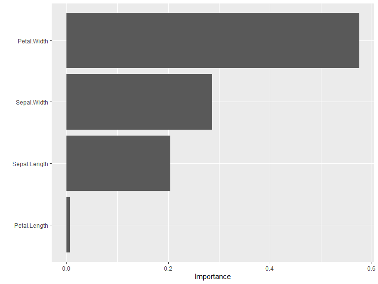
Note: Weight caching increases memory usage proportional to network size. Only enable it when you plan to compute variable importance multiple times on the same model.
Falbel D, Luraschi J (2023). torch: Tensors and Neural Networks with ‘GPU’ Acceleration. R package version 0.13.0, https://torch.mlverse.org, https://github.com/mlverse/torch.
Wickham H (2019). Advanced R, 2nd edition. Chapman and Hall/CRC. ISBN 978-0815384571, https://adv-r.hadley.nz/.
Goodfellow I, Bengio Y, Courville A (2016). Deep Learning. MIT Press. https://www.deeplearningbook.org/.
MIT + file LICENSE
Please note that the kindling project is released with a Contributor Code of Conduct. By contributing to this project, you agree to abide by its terms.