Item response theory (IRT) has become a standard method in the analysis of survey assessment data. In the IRT paradigm, the performance of test takers (i.e., their capacity to answer a question correctly) is explained by individual ability and the properties or characteristics of the test. Classically, ability is assumed to be 1) univariate and 2) homogenous across person characteristics. First, ability, which is a placement of each test taker on a continuum, can often be explained by heterogeneity among study participants. Second, recent applications involve characterizing a general, higher-order, ability which explain multiple, first-order, domains of ability. The natural progression, then, is to explain the heterogeneity of general ability. The open-source R package hlt implements the random-walk Metropolis-Hastings algorithm to estimate the higher-order IRT model by implementing a flexible Bayesian framework. We implement a higher-order generalize partial credit model and its extension of latent regression with the goal of explaining the relationship between the general latent construct and a set of explanatory variables.
The most recent hlt release can be installed from CRAN via
install.packages("hlt")The most recent hlt development release can be installed from Github via devtools. If you do not have devtools installed on your system, go here to install it.
install.packages("devtools")devtools::install_github("mkleinsa/hlt")Once installed, load the package with
library("hlt")The R package hlt requires R (version > 3.5.0) and Rcpp (≥ 0.12.0). Pre-build binaries for the current official release of the package are available from CRAN (Comprehensive R Archive Network), but if the user desires to compile the package for himself, then the typical R compiler tools will have to be installed. Instructions can be found on the R Project’s website at https://www.r-project.org/nosvn/pandoc/devtools.html.
The latest development version of the package can be found on Github (https://github.com/mkleinsa/hlt). The development version contains updates to the software which are typically a few weeks ahead of the CRAN release. The hlt package can be installed from CRAN and loaded via the R console with the following commands:
install.packages(“hlt”)
library(hlt)
To install the development version of hlt, install the devtools package (Wickham et al., 2021) and run the following command:
devtools::install_github(“mkleinsa/hlt”)
library(hlt)
See the README of the hlt package on the Github repository page for additional details about package installation. To install the development version of the package, compilation of the C++ code is required at install, so the user’s development toolchain must at least include a C++ compiler.
The main model fitting function, hlt(), encapsulates all of the package’s estimation procedures. The output is either an object of class hltObj for a single run or an hltObjList for multiple parallel runs. For each object class, R generics are available to print(), plot(), produce a summary() or merge chains (merge_chains()) to merge multiple parallel runs.
The hlt package includes a function to simulate data under each of the modeling scenarios. In this section, we demonstrate how to simulate data and estimate the correct higher-order IRT model. For full documentation of the simulation function with examples, run ?hltsim at the R console.
The hltsim function has arguments for the type of higher-order IRT model (type), the sample size (n), the number of latent domains (ntheta), the true loadings for each latent domain (lambda), the domain membership of each latent domain (id), the number of levels of each question (dL), the number of regression parameters (nB), and the true regression parameter values (beta). To simulate the generalized partial credit model without regression, the function call is as follows:
xdat = hltsim(n = 250, type = "2p", ntheta = 4,
  lambda = c(0.5, 0.8, 0.9, 0.4), id = c(rep(0, 15),
   rep(1, 15), rep(2, 15), rep(3, 15)), dL = 2)
In this example, we simulate data for 250 participants from a survey measuring four domains with 15 items per domain. Each response is binary, yes/no (1 or 0). In the following sections, we will demonstrate the other features of hltsim in demonstrating the modeling procedures.
The hltsim function returns a named list of simulated outputs and arguments including the simulated survey data (x), regression design matrix (z), parameter settings (s.lambda, s.alpha, s.delta, s.beta), and domain I.D. vector (id).
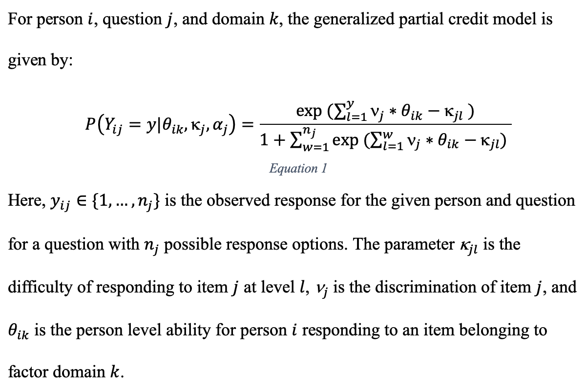
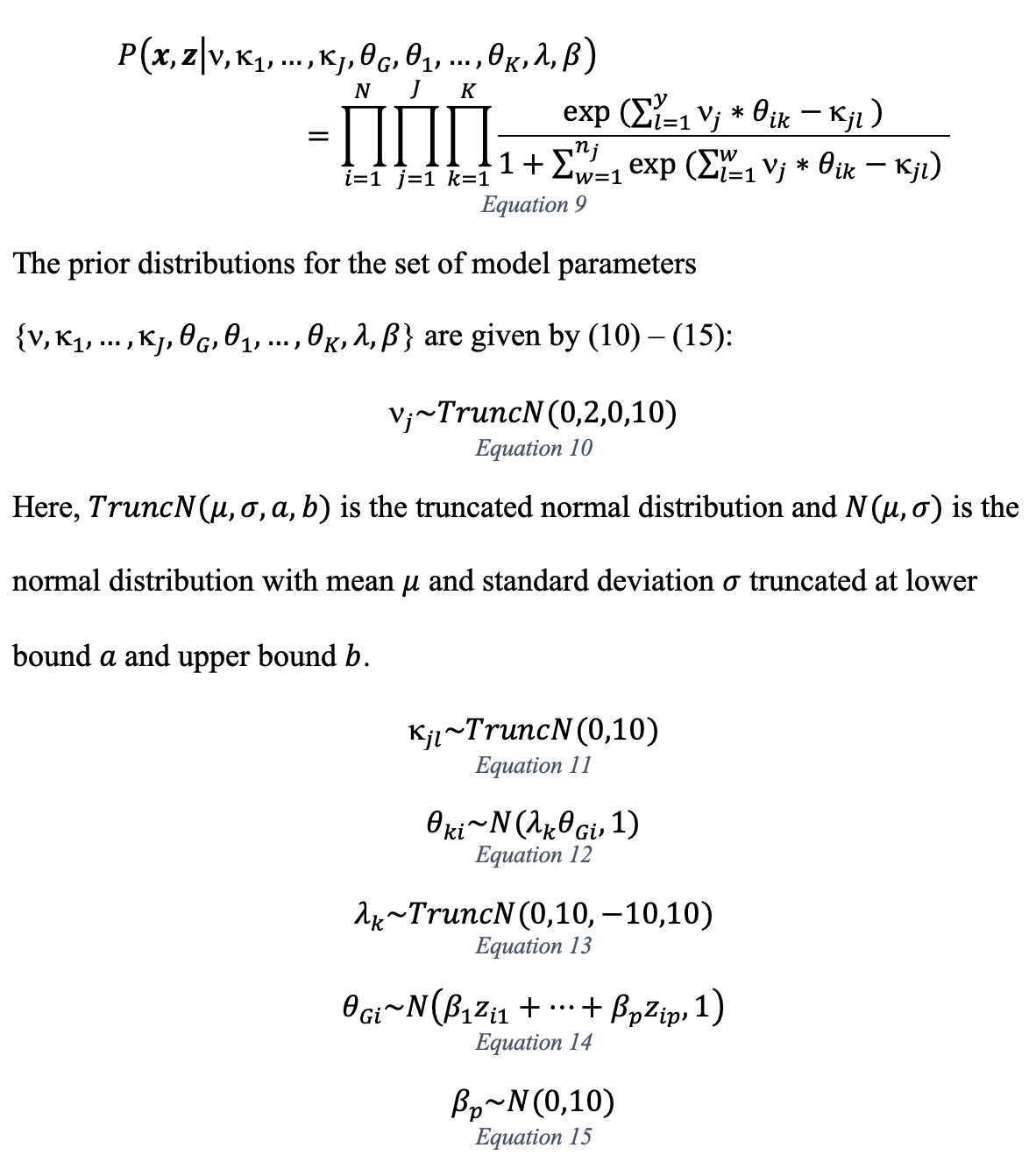
The descriptive higher-order item response theory model has two components: a measurement model which describes the probability of responding correctly to the given survey item; and a factor structure model which describes the relationship between the general factor and domain specific factors.
We focus on the partial credit model (PCM) and the generalized partial credit model (GPCM) for their flexibility (Muraki, 1992; Masters, 1982). The PCM and GPCM are flexible enough to account for dichotomous and polytomous response items, covering a wide variety of survey question types. In the dichotomous case, the PCM model is mathematically equivalent to the 1-parameter logistic model and the GPCM is equivalent to the 2-parameter logistic model. Thus, four different types IRT measurement models can be fit with this package, and any number of dichotomous and polytomous item types is possible.
The following R code fits the HO-IRT model to the simulated data set:
mod1 = hlt(x = xdat$x, id = xdat$id, iter = 12e5,
  burn = 6e5, delta = 0.023)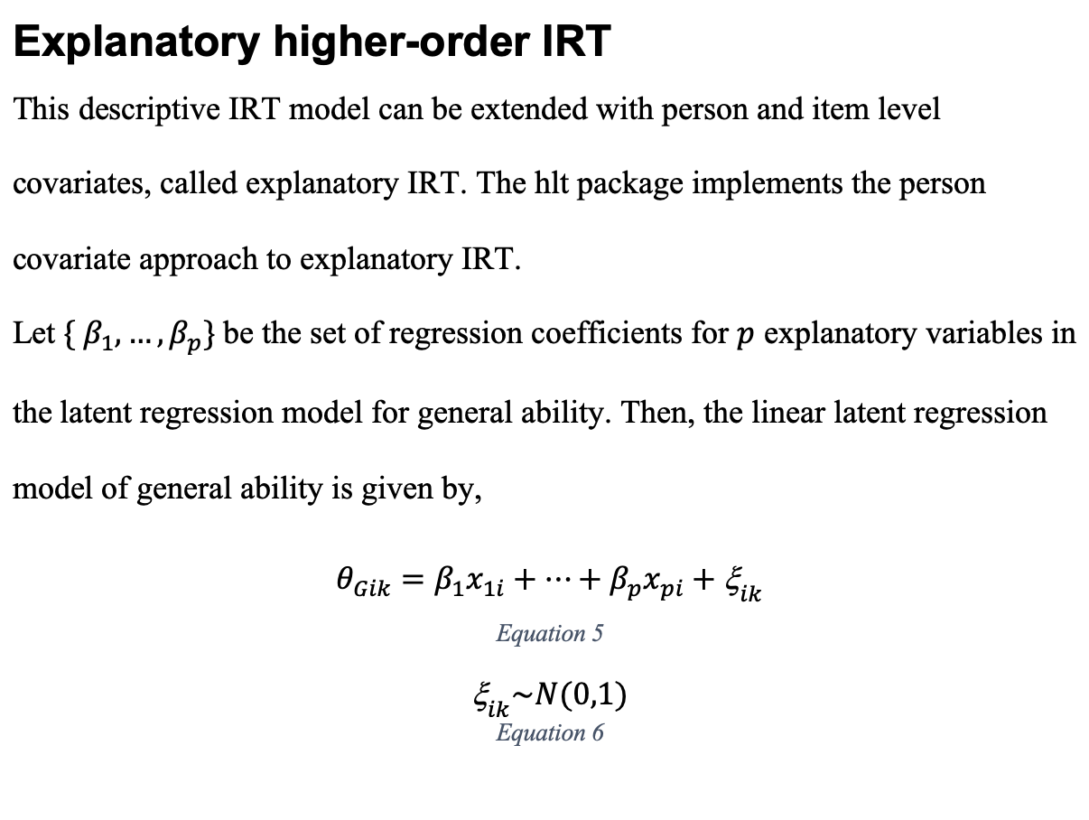
To adapt the previous simulation to include latent regression, the function call is as follows:
xdat = hltsim(n = 250, type = "2p", ntheta = 4,
  lambda = c(0.5, 0.8, 0.9, 0.4), id = c(rep(0, 15),
  rep(1, 15), rep(2, 15), rep(3, 15)), dL = 2,
  beta = c(0.5, -0.7), nB = 2)
Note that two arguments were added: beta = c(0.5, -0.7), which sets two new regression coefficients, and nB = 2, which signifies the number of regression coefficients set. The corresponding hlt call to fit the model is:
mod2 = hlt(x = xdat$x, id = xdat$id, z = xdat$z,
  iter = 12e5, burn = 6e5, delta = 0.023, nchains = 1)
The adult self-transcendence inventory, or ASTI, was originally created to assess the construct of wisdom through self-transcendence (Levenson et al., 2005). Recently, Koller et al. (2017) re-analyzed 24 ASTI items measuring self-transcendence over five dimensions. The five domains of the Koller ASTI survey were: 1) self-knowledge and integration (four items); 2) peace of mind (four items); 3) non-attachment (four items); 4) self-transcendence (seven items); 5) and presence in the here-and-now and growth (six items).
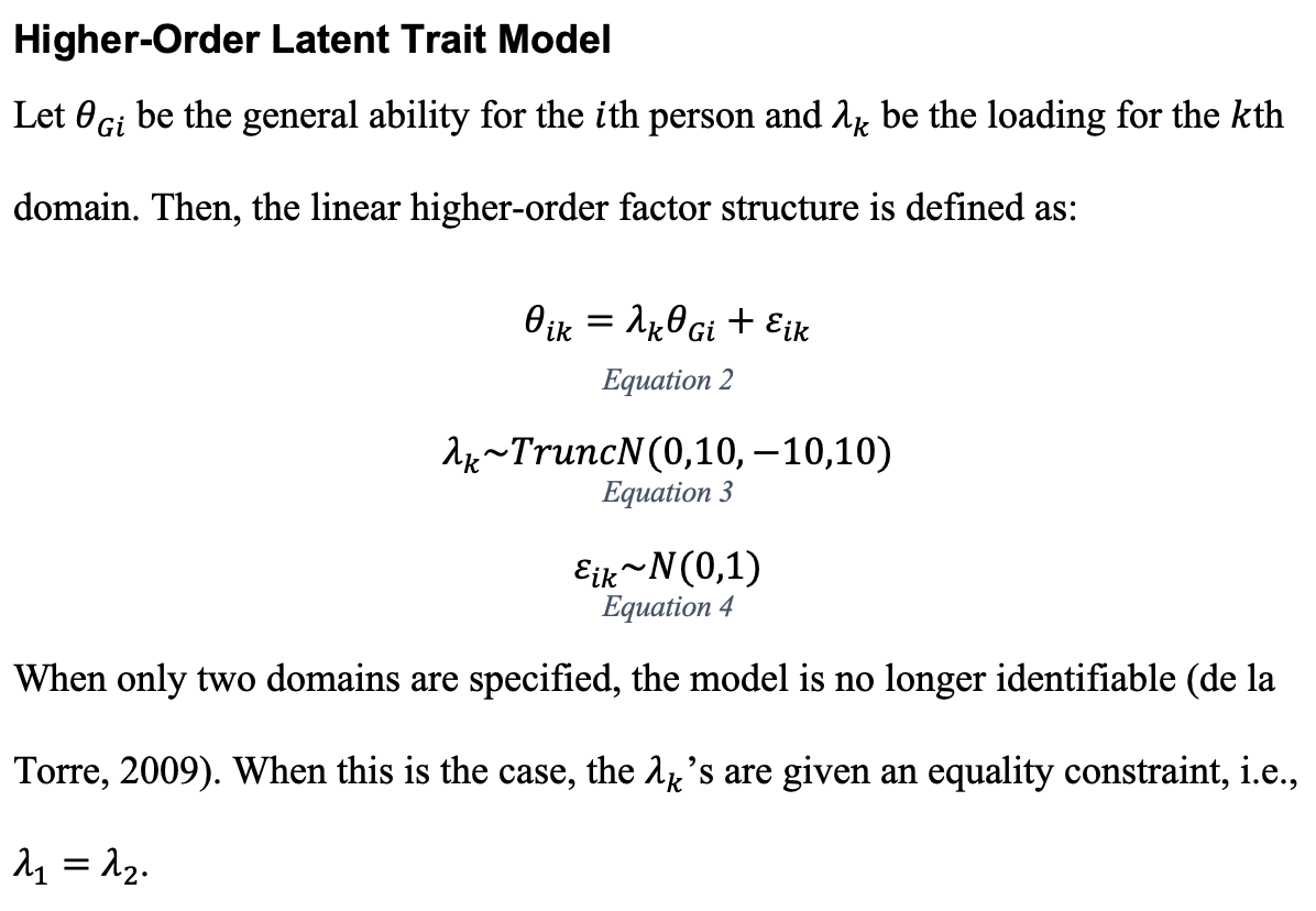
A primary goal of the study was to determine if the ASTI formed a unidimensional scale. However, since the five dimension each form their own theoretical domain of wisdom, a unidimensional scale may be an oversimplification of the problem. This is further supported by the fact that the authors found that a multidimensional IRT (M-IRT) model with five dimensions fit the data better than the univariate model. Higher-order IRT (HO-IRT) tests the correct hypothesis if what is sought is a single general dimension governing the hypothesized five domains of wisdom.
In this example, we demonstrate the process of fitting the generalized partial credit HO-IRT (descriptive) model to the ASTI data and we assess the effect of gender (male/female) and student status (student/non-student) on the higher-order transcendence dimension using the HO-IRT-LR (explanatory) model. For a graphical representation of the HO-IRT-LR model of the ASTI data, refer to Figure 1.
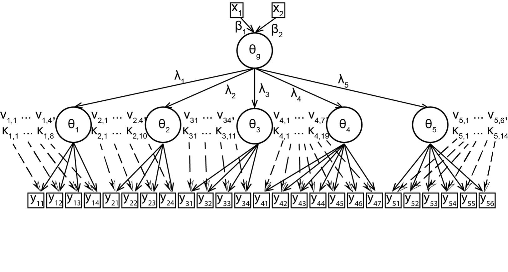
Figure 1. Higher-Order IRT Latent Regression Diagram for ASTI Data. Rectangles represent observed data, circles represent latent data, and the other parameters are left not circled. The notation used here matches Eq. 1.
Data preparation The publicly available data set comes from the R package MPsychoR on CRAN (Mair 2018), but it is also available through the hlt package with:
library(hlt)
data(“asti”)
Preparing the Input The model fitting procedure occurs in two stages: first we do a single chain run of the algorithm to tune the acceptance rate and to monitor convergence. Once convergence is achieved, we use the starting values from the previous solution and run three parallel chains. Finally, the results are summarized. The hlt model fitting function requires that survey responses from a given question i are integers ranging from 0 to n -1. However, the ASTI data are coded from 1,…,n, so the responses are adjusted with:
x = asti[, 1:25] - 1The id vector for the ASTI data requires 5 unique integer levels (one level for each domain of the survey) again coded from 0 to k-1:
id = c(rep(0, 4), rep(1, 4), rep(2, 4), rep(3, 7), rep(4, 6))Note that the values of id must be an ordered sequence and the domain cannot overlap, e.g., c(0,0,0,1,0,0,1,1) is invalid and should rather be c(0,0,0,0,0,1,1,1). Lastly, in preparation for the latent regression analysis, we create a matrix of dummy variables for each variable included:
z = asti[, 26:27]
z[, 1] = (z[, 1] == "students") * 1
z[, 2] = (z[, 2] == "male") * 1
Notice that this example includes two factor which each have two levels, thus 2 – 1 dummy variables are required of each variable. For continuous variables, a singe numeric vector is required, but that each numeric variable also be standardized.
Model Fitting We first conduct a descriptive analysis to assess the fit of the HO-IRT model in terms of the item parameters using the GPCM. We then fit the HO-IRT-LR model to estimate the latent regression coefficients. While the analysis did not need to proceed in stages, it was done to show the software’s capacity for both facets if IRT.
Descriptive Analysis In the descriptive case, we seek to describe the properties of each scale within the context of a higher-order latent trait structure. These properties are characterized by the item parameters of discrimination and difficulty. Without prior knowledge about an acceptable proposal variance or starting values that are reasonably close to the posterior mode, we first need to tune the sampler and then sample until the posterior mode stops changing. Then, for the final run, we provide a set of starting values and run n parallel chains, check the trace plots, merge the chains, and summarize the results. We first ran the model at 1e2, 1e3, 1e4, respective numbers of iterations, tuning the proposal variance parameter delta. Once an acceptance rate of approximately 0.234 was achieved, we ran one chain until the posterior mode was reached. Then, we ran three chains using the single chain starting values. The model fitting script is as follows:
asti_gpc = hlt(x = x, id = id, iter = 2.5e6, burn = 2e6,
    delta = 0.01, type = "2p")

Higher-order item response theory model with 5 first-order domains
 Total number of parameters: 6879
 Model type (1p = "Partial Credit model"; 2p = "Generalized Partial Credit Model"): 2p
 iterations: 2500000; burn-in: 2e+06
 Proposal standard deviation: 0.01
 Acceptance rate: 0.225

Loadings:  1.276 1.537 0.43 0.285 1.712
asti_gpc_m = hlt(x = x, id = id, iter = 2e5, burn = 1e5,
delta = 0.01, type = "2p", nchains = 3,
start = get_hlt_start(asti_gpc, nchains = 3)) It is essential that the MCMC chains are monitored for convergence. Once a model is fitted trace plots for the parameters should be checked individually with:
plot(asti_gpc_m, param = "lambda4", type = "trace")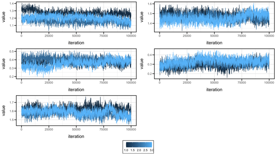
Figure 2. Traceplots of the five latent factor loadings. Traces are shown for post burn-in iterations for lambda1 (top left), lambda2 (top right), lambda3 (middle left), lambda4 (middle right), and lambda5 (bottom left).
Figure 2 displays the MCMC chains for four selected parameters. For a complete set of parameter names in the model, use colnames(asti_gpc$post). Next, we show how to view the item level parameter estimates using the model summary function after merging the multiple chains:
asti_merg = merge_chains(asti_gpc_m)
summary(asti_merg, param = "alpha")
summary(asti_merg, param = "delta")
The item characteristic, item information, and total information curves are produced with the following code (see Figure 3, below):
plot(asti_merg, item = 1, type = "icc", min = -6, max = 6)
plot(asti_merg, item = 1, type = "iic", min = -6, max = 6)
plot(asti_merg, item = 1, type = "tic", min = -6, max = 6)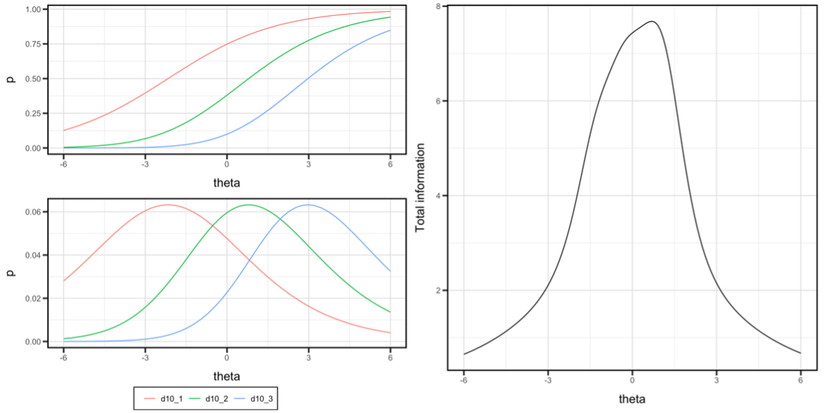
Figure 3. Item characteristic curve for item 1 (top left), item information curve for item 1 (bottom left), and total information curve (right).
The relationship between latent dimension can be characterized by the raw factor loadings, correlations between the general factor and each first-order domain, and the correlations among the first-order domains themselves, as shown below and in Figure 4:
summary(asti_merg, param = "lambda")

         mean    se  2.5%   50% 97.5%
lambda1 1.209 0.059 1.105 1.207 1.326
lambda2 1.464 0.038 1.389 1.464 1.540
lambda3 0.376 0.042 0.287 0.378 0.453
lambda4 0.313 0.039 0.236 0.313 0.387
lambda5 1.595 0.044 1.511 1.595 1.682summary(asti_merg, param = "correlation")
theta1 theta2 theta3 theta4 theta5 theta6
theta1 1.000 0.787 0.406 0.281 0.824 0.895
theta2 0.787 1.000 0.477 0.344 0.853 0.937
theta3 0.406 0.477 1.000 0.236 0.427 0.510
theta4 0.281 0.344 0.236 1.000 0.367 0.402
theta5 0.824 0.853 0.427 0.367 1.000 0.951
theta6 0.895 0.937 0.510 0.402 0.951 1.000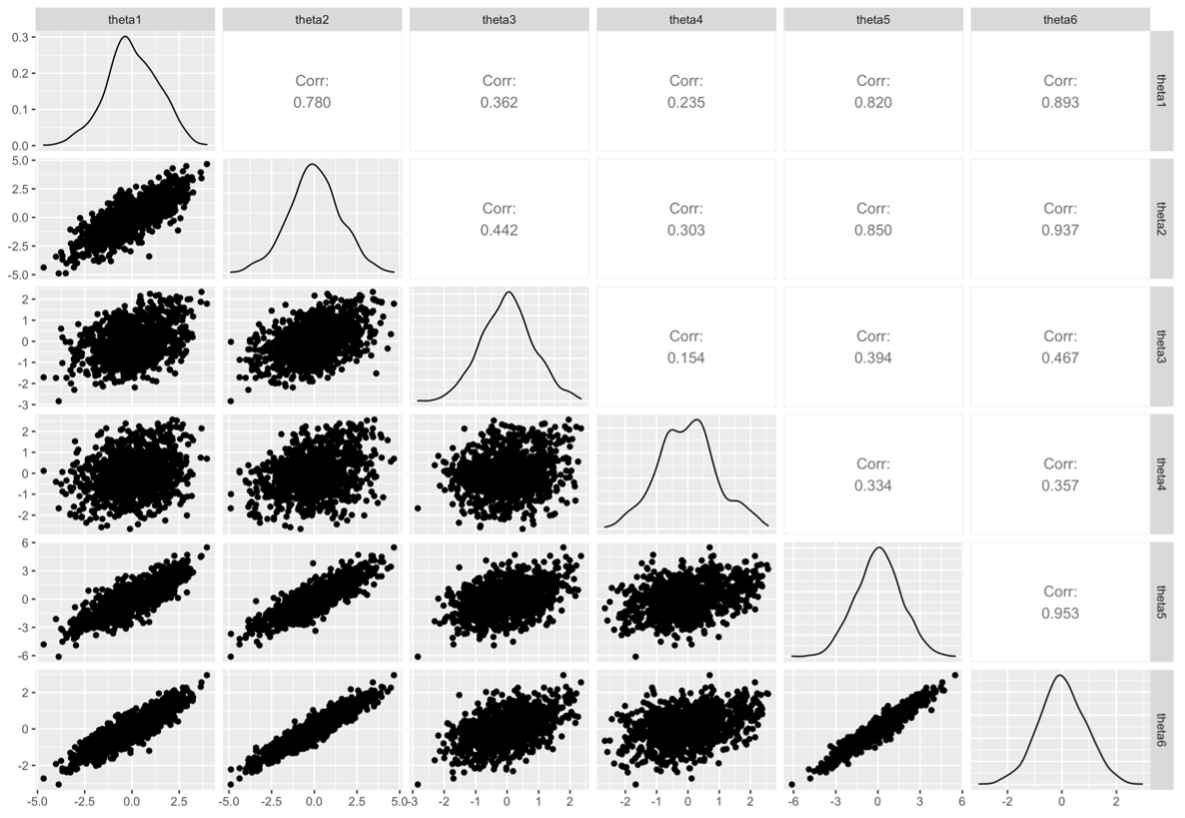
Figure 4. Correlogram showing the bivariate correlations (upper triangle), scatter plots (lower triangle), and density plots (diagonal) for each first-order domain (theta1 through theta5) and the higher-order domain (theta6).
The ability estimates are extracted with summary for each of the first-order domains and the higher-order domain. Since there are five first-order domains, dimension = 1,…,5 will give each respective summary, and dimension = 6 givens the higher order abilities:
# First dimension
summary(asti_merg, param = "theta", dimension = 1)
# higher-order dimension
summary(asti_merg, param = "theta", dimension = 6)
Explanatory Analysis In the explanatory case, the person characteristics of gender and student status are used to explain heterogeneity in the ability of persons to answer questions correctly. This analysis is much simpler given the work we did in the descriptive analysis, which provided good starting values and proposal variance. Now, we repeat the previous analysis, but this time by also specifying a latent regression model:
asti_gpc_reg = hlt(x = x, id = id, z = z, iter = 2.5e6,
  burn = 2e6, delta = 0.01, type = "2p",
  start = get_hlt_start(asti_merg, nchains = 1),
  nchains = 1)
asti_gpc_reg
Higher-order item response theory model with 5 first-order domains
 Total number of parameters: 6881
 Model type (1p = "Partial Credit model"; 2p = "Generalized Partial Credit Model"): 2p
 iterations: 2500000; burn-in: 2e+06
 Proposal standard deviation: 0.01
 Acceptance rate: 0.205

Loadings:  1.443 1.517 0.49 0.244 1.579
Latent regression beta estimates:  -0.118 -0.058
asti_gpc_reg_m = hlt(x = x, id = id, z = z, iter = 1e6,
burn = 5e5, delta = 0.01, type = "2p",
start = get_hlt_start(asti_gpc_reg, nchains = 3),
nchains = 3)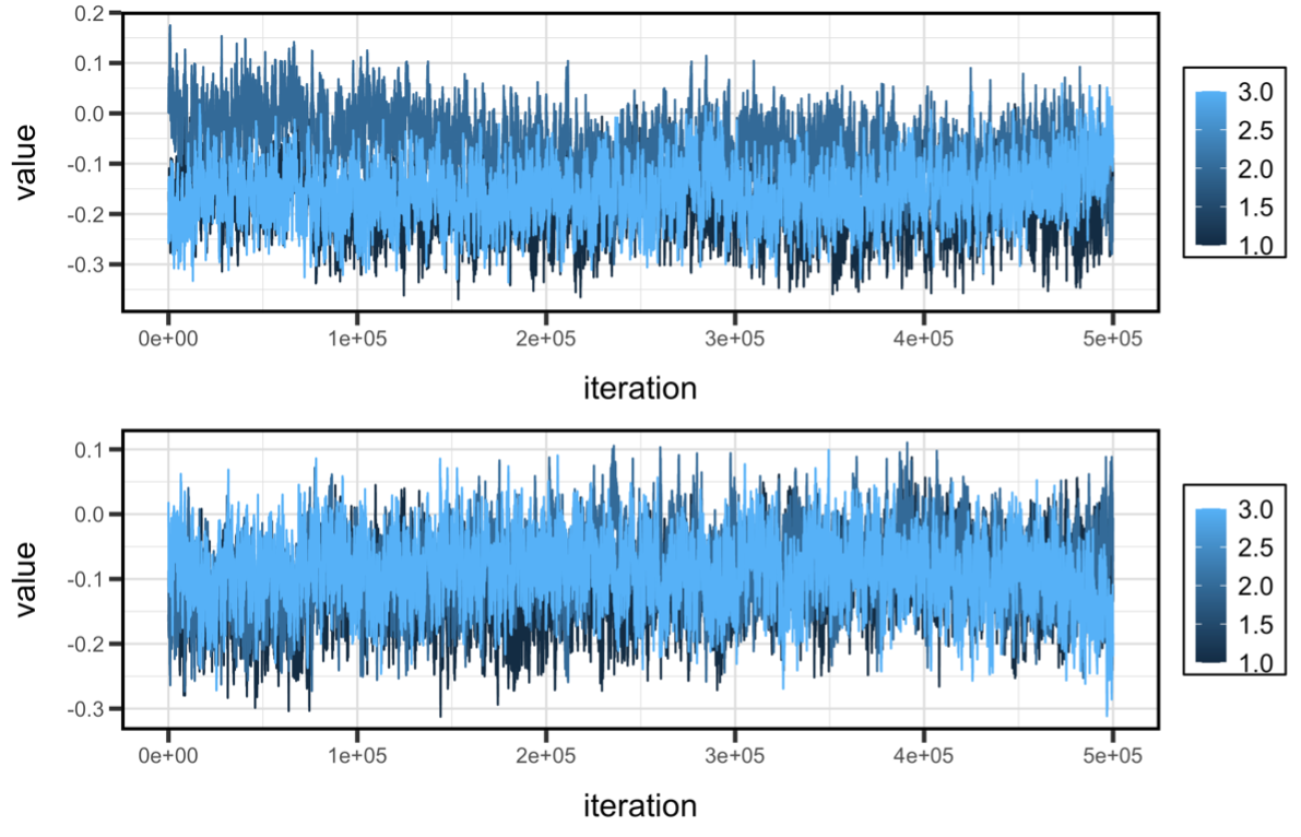
Figure 5. Traceplots of latent regression coefficients. Traces are shown for post burn-in iterations for beta1 (top) and beta2 (bottom). Beta1 represents “students” and beta2 represents “males”.
We then merge the chains into one summary and inspect the results:
asti_gpc_reg_mm = merge_chains(asti_gpc_reg_m)
summary(asti_gpc_reg_mm, param = "beta")

        mean    se   2.5%    50% 97.5%
beta1 -0.137 0.076 -0.272 -0.143 0.023
beta2 -0.096 0.053 -0.201 -0.095 0.008If you are interested in contributing to the development of hlt please open an issue to request.
Paper under review. See the vignettes/ folder for a PDF
of the manuscript.