![]()
gwid is an R-package designed for the analysis of IBD (Identity by Descent) data, to discover rare alleles (susceptibility regions) associated with case-control phenotype. Although Genome Wide Association Studies (GWAS) successfully reveal numerous common variants linked to diseases, they exhibit lack of power to identify rare alleles. To address this limitation, we have developed a pipeline that employs IBD data (output of refined-IBD software). This methodology encompasses a sequential process for analyzing the aforementioned data within isolated populations. The primary objective of this approach is to enhance the sensitivity of variant detection by utilizing information from genetically related individuals, thereby facilitating the identification of causal variants. An overall representation of the pipeline is visually depicted in the following figure.
gwid pipeline
The gwid package receives four types of inputs: a
genotype file, an IBD file, a haplotype file, and phenotype file. The
genotype data is derived from the output of the SNPRelate
package in the form of a gds file. The IBD file takes
the form of tabulated data produced by the Refined
IBD software. Haplotype file comes from the output of the Beagle,
while phenotype data is represented using an R list.
You can install the stable version of gwid from CRAN with:
if (!require("BiocManager", quietly = TRUE))
    install.packages("BiocManager")

BiocManager::install(c("SNPRelate","gdsfmt"))
install.packages("gwid")
Alternatively, you can install the stable version of
gwid with:
if (!require("BiocManager", quietly = TRUE))
    install.packages("BiocManager")

BiocManager::install("gwid")
Also, you can install the development version of gwid
from GitHub with:
if (!require("devtools", quietly = TRUE))
    install.packages("devtools")

devtools::install_github("soroushmdg/gwid")We demonstrated the key functionalities of gwid using the rheumatoid
arthritis (RA) GWAS dataset. This dataset consisted of DNA samples
collected from 478 individuals diagnosed with rheumatoid arthritis (RA)
and a control group of 1,434 individuals without RA. Genotyping was
performed using the Illumina Infinium array. All samples were obtained
from a genetically homogeneous population in central Wisconsin
exhibiting elevated relatedness structure. Because size of data is
large, we use pggyback package to upload and download data
from github repository.
# install.packages("piggyback")
piggyback::pb_download(repo = "soroushmdg/gwid",
            tag = "v0.0.1",
            dest = tempdir())
ibd_data_file <- paste0(tempdir(),"//chr3.ibd")
genome_data_file <- paste0(tempdir(),"//chr3.gds")
phase_data_file <- paste0(tempdir(),"//chr3.vcf")
case_control_data_file <- paste0(tempdir(),"//case-cont-RA.withmap.Rda")In this code we explain each input data files individually.
case_control is object of class caco that has
phenotype information. snp_data_gds object of class
gwas read output of SNPRelate package, we use
this package because it is very fast and efficient.
haplotype_data object of class phase has
haplotype data. ibd_data is an object of gwid
class that has IBD information.
library(gwid)
#>
#> Attaching package: 'gwid'
#> The following objects are masked from 'package:base':
#>
#>     print, subset

# case-control data
case_control <- gwid::case_control(case_control_rda = case_control_data_file)
names(case_control) # cases and controls group
#> [1] "cases" "case1" "case2" "cont1" "cont2" "cont3"
summary(case_control) # in here, we only consider cases,cont1,cont2,cont3
#>       Length Class  Mode
#> cases 478    -none- character
#> case1 178    -none- character
#> case2 300    -none- character
#> cont1 477    -none- character
#> cont2 478    -none- character
#> cont3 478    -none- character
# groups in the study
case_control$cases[1:3] # first three subject names of cases group
#> [1] "MC.154405@1075678440" "MC.154595@1075642175" "MC.154701@1076254706"

# read SNP data (use SNPRelate to convert it to gds) and count number of
# minor alleles
snp_data_gds <- gwid::build_gwas(gds_data = genome_data_file,
                                 caco = case_control,
                                 gwas_generator = TRUE)
class(snp_data_gds)
#> [1] "gwas"
names(snp_data_gds)
#> [1] "smp.id"   "snp.id"   "snp.pos"  "smp.indx" "smp.snp"  "caco"     "snps"
# it has information about counts of minor alleles in each location.
head(snp_data_gds$snps)
#> Key: <snp_pos>
#>    snp_pos case_control value
#>      <int>       <fctr> <int>
#> 1:   66894        cases   627
#> 2:   66894        case1   240
#> 3:   66894        case2   387
#> 4:   66894        cont1   639
#> 5:   66894        cont2   647
#> 6:   66894        cont3   646

# read haplotype data (output of beagle)
haplotype_data <- gwid::build_phase(phased_vcf = phase_data_file,
                                    caco = case_control)
class(haplotype_data)
#> [1] "phase"
names(haplotype_data)
#> [1] "Hap.1" "Hap.2"
dim(haplotype_data$Hap.1) # 22302 SNP and 1911 subjects
#> [1] 22302  1911

# read IBD data (output of Refined-IBD)
ibd_data <- gwid::build_gwid(ibd_data = ibd_data_file,
                             gwas = snp_data_gds)
class(ibd_data)
#> [1] "gwid"
ibd_data$ibd # refined IBD output
#>                              V1    V2                      V3    V4    V5
#>                          <char> <int>                  <char> <int> <int>
#>      1: MC.AMD127769@0123889787     2    MC.160821@1075679055     1     3
#>      2: MC.AMD127769@0123889787     1 MC.AMD107154@0123908746     1     3
#>      3: MC.AMD127769@0123889787     2    9474283-1-0238040187     1     3
#>      4: MC.AMD127769@0123889787     1    MC.159487@1075679208     2     3
#>      5:    MC.163045@1082086165     2    MC.160470@1075679095     1     3
#>     ---
#> 377560:    1492602-1-0238095971     2    2235472-1-0238095471     2     3
#> 377561:    4618455-1-0238095900     2    3848034-1-0238094219     1     3
#> 377562:    MC.160332@1075641581     2    9630188-1-0238038787     2     3
#> 377563: MC.AMD122238@0124011436     2    MC.159900@1076254946     1     3
#> 377564: MC.AMD105910@0123907456     1    7542312-1-0238039298     1     3
#>                V6        V7    V8    V9
#>             <int>     <int> <num> <num>
#>      1:  32933295  34817627  3.26 1.884
#>      2:  29995340  31752607  4.35 1.757
#>      3:  34165785  35898774  6.36 1.733
#>      4:  21526766  23162240  8.71 1.635
#>      5:  11822616  13523010  5.29 1.700
#>     ---
#> 377560: 194785443 196328849  4.92 1.543
#> 377561: 190235788 192423862  7.77 2.188
#> 377562: 184005719 186184328  5.95 2.179
#> 377563: 181482803 184801115  3.58 3.318
#> 377564: 182440135 183972729  3.03 1.533
ibd_data$res # count number of IBD for each SNP location
#>           snp_pos case_control value
#>             <num>       <fctr> <num>
#>      1:     66894        cases    27
#>      2:     82010        cases    28
#>      3:     89511        cases    29
#>      4:    104972        cases    29
#>      5:    107776        cases    29
#>     ---
#> 133808: 197687252        cont3    44
#> 133809: 197701913        cont3    44
#> 133810: 197744198        cont3    44
#> 133811: 197762623        cont3    44
#> 133812: 197833758        cont3    44
plot methodThe plot function can be applied to the
gwid class to display the counts of IBD in each Single SNP
among both case and control groups. By utilizing the
ly=TRUE parameter, the user has the option to transform the
plot into a plotly object, facilitating interactive
exploration of the entire chromosome or specific regions of interest
through the use of snp_start and snp_end
parameters. Additionally, the y parameter enables the
inclusion of only specific groups of subjects for consideration.
# plot count of IBD in chromosome 3
plot(ibd_data,y = c("cases","cont1"),
ly = FALSE) 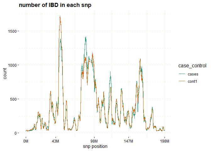
# Further investigate location between 117M and 122M
# significant number of IBD's in group cases, compare to cont1, cont2 and cont3.
plot(ibd_data,
     y = c("cases","cont1"),
     snp_start = 117026294,
     snp_end = 122613594,
ly = FALSE) 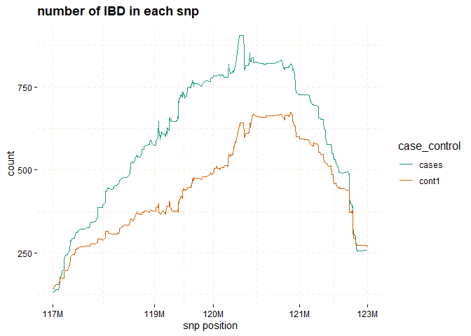
Through the utilization of the fisher_test method, it
becomes possible to calculate p-values within chosen regions. These
p-values help assess whether there are noteworthy differences in counts
between the case and control groups.
model_fisher <- gwid::fisher_test(ibd_data,case_control,
                                  reference = "cases",
                                  snp_start = 117026294,
                                  snp_end = 122613594)

class(model_fisher)
#> [1] "test_snps"  "data.table" "data.frame"

plot(model_fisher,
     y = c("cases","cont1"),
     ly = FALSE)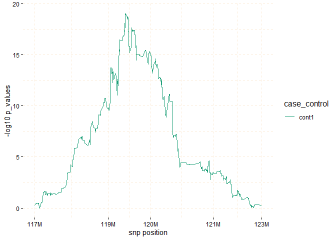
You can perform permutation test as follows:
model_permutation <- gwid::permutation_test(ibd_data,gwas = snp_data_gds,
                                            reference = "cases",
                                            snp_start = 117026294,
                                            snp_end = 122613594,
                                            nperm = 10000)
plot(model_permutation)
The haplotype_structure method can be utilized to
extract haplotypes from regions that exhibit IBD patterns in a sliding
window manner. w is length of sliding window and
hap_str <- gwid::haplotype_structure(ibd_data,
phase = haplotype_data,
w = 10,
snp_start = 117026294,snp_end = 122613594)
class(hap_str)
#> [1] "haplotype_structure" "data.table" "data.frame"
hap_str[sample(1:nrow(hap_str),size = 5),] # structures column have haplotype of length w=10
#> case_control snp_pos window_number smp structures
#> <fctr> <num> <int> <char> <char>
#> 1: case1 120147864 414 MC.AMD117897@0123890753 0011101011
#> 2: case2 119694893 368 MC.AMD116754@0123911408 0000000001
#> 3: cont1 117383670 41 MC.157186@1075678676 0000000001
#> 4: cont2 122353931 721 MC.AMD134768@0123911507 0000001001
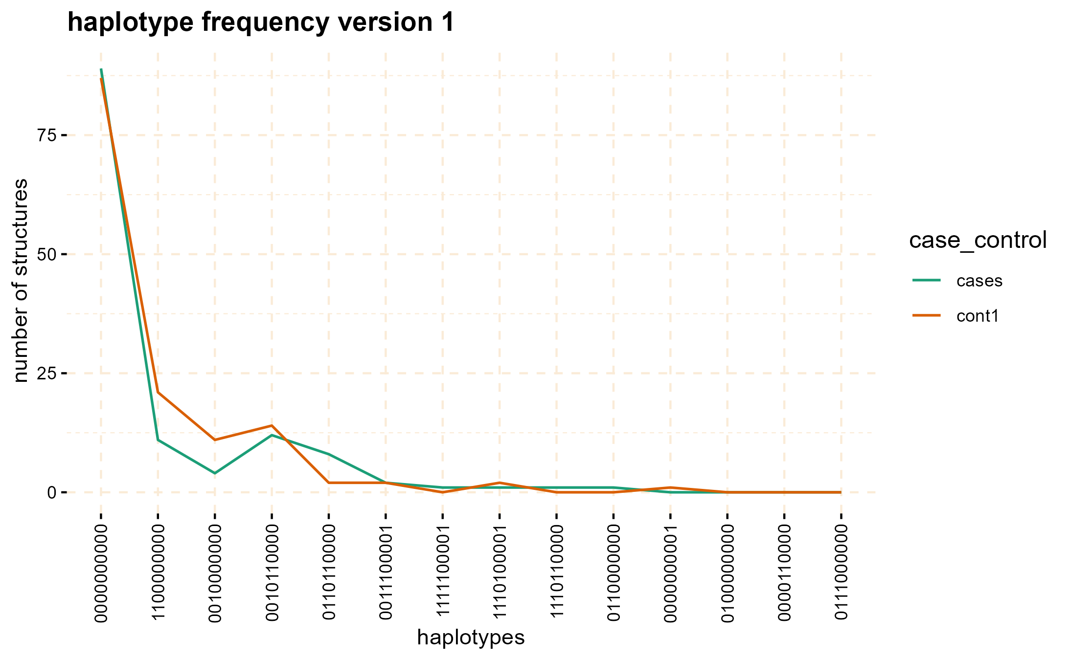
#> 5: cont2 122089359 676 MC.158775@1075642103 1000000000The haplotype_frequency method can be employed to
extract the count of these structures, which can then be plotted for
each window.
haplo_freq <- gwid::haplotype_frequency(hap_str)
# plot haplotype counts in first window (nwin=1).
 plot(haplo_freq,
   y = c("cases", "cont1"),
   plot_type = "haplotype_structure_frequency",
   nwin = 1, type = "version1",
   ly = FALSE
 )