![]()
![]()
![]()
Tidy, analyze, and plot causal directed acyclic graphs (DAGs).
ggdag uses the powerful dagitty package to
create and analyze structural causal models and plot them using
ggplot2 and ggraph in a consistent and easy
manner.
You can install ggdag with:
install.packages("ggdag")Or you can install the development version from GitHub with:
# install.packages("devtools")
devtools::install_github("r-causal/ggdag")ggdag makes it easy to use dagitty in the
context of the tidyverse. You can directly tidy dagitty
objects or use convenience functions to create DAGs using a more R-like
syntax:
library(ggdag)
library(ggplot2)

#  example from the dagitty package
dag <- dagitty::dagitty("dag {
    y <- x <- z1 <- v -> z2 -> y
    z1 <- w1 <-> w2 -> z2
    x <- w1 -> y
    x <- w2 -> y
    x [exposure]
    y [outcome]
  }")

tidy_dag <- tidy_dagitty(dag)

tidy_dag
#> # A DAG with 7 nodes and 12 edges
#> #
#> # Exposure: x
#> # Outcome: y
#> #
#> # A tibble: 13 × 8
#>    name       x      y direction to       xend   yend circular
#>    <chr>  <dbl>  <dbl> <fct>     <chr>   <dbl>  <dbl> <lgl>
#>  1 v     0.496  -3.40  ->        z1     1.83   -2.92  FALSE
#>  2 v     0.496  -3.40  ->        z2     0.0188 -2.08  FALSE
#>  3 w1    1.73   -1.94  ->        x      2.07   -1.42  FALSE
#>  4 w1    1.73   -1.94  ->        y      1.00   -0.944 FALSE
#>  5 w1    1.73   -1.94  ->        z1     1.83   -2.92  FALSE
#>  6 w1    1.73   -1.94  <->       w2     0.873  -1.56  FALSE
#>  7 w2    0.873  -1.56  ->        x      2.07   -1.42  FALSE
#>  8 w2    0.873  -1.56  ->        y      1.00   -0.944 FALSE
#>  9 w2    0.873  -1.56  ->        z2     0.0188 -2.08  FALSE
#> 10 x     2.07   -1.42  ->        y      1.00   -0.944 FALSE
#> 11 y     1.00   -0.944 <NA>      <NA>  NA      NA     FALSE
#> 12 z1    1.83   -2.92  ->        x      2.07   -1.42  FALSE
#> 13 z2    0.0188 -2.08  ->        y      1.00   -0.944 FALSE

#  using more R-like syntax to create the same DAG
tidy_ggdag <- dagify(
  y ~ x + z2 + w2 + w1,
  x ~ z1 + w1 + w2,
  z1 ~ w1 + v,
  z2 ~ w2 + v,
  w1 ~ ~w2, # bidirected path
  exposure = "x",
  outcome = "y"
) %>%
  tidy_dagitty()

tidy_ggdag
#> # A DAG with 7 nodes and 12 edges
#> #
#> # Exposure: x
#> # Outcome: y
#> #
#> # A tibble: 13 × 8
#>    name      x     y direction to     xend  yend circular
#>    <chr> <dbl> <dbl> <fct>     <chr> <dbl> <dbl> <lgl>
#>  1 v     -3.58  3.30 ->        z1    -4.05  4.63 FALSE
#>  2 v     -3.58  3.30 ->        z2    -2.23  3.74 FALSE
#>  3 w1    -3.03  5.74 ->        x     -3.20  5.14 FALSE
#>  4 w1    -3.03  5.74 ->        y     -1.98  5.22 FALSE
#>  5 w1    -3.03  5.74 ->        z1    -4.05  4.63 FALSE
#>  6 w1    -3.03  5.74 <->       w2    -2.35  4.72 FALSE
#>  7 w2    -2.35  4.72 ->        x     -3.20  5.14 FALSE
#>  8 w2    -2.35  4.72 ->        y     -1.98  5.22 FALSE
#>  9 w2    -2.35  4.72 ->        z2    -2.23  3.74 FALSE
#> 10 x     -3.20  5.14 ->        y     -1.98  5.22 FALSE
#> 11 y     -1.98  5.22 <NA>      <NA>  NA    NA    FALSE
#> 12 z1    -4.05  4.63 ->        x     -3.20  5.14 FALSE
#> 13 z2    -2.23  3.74 ->        y     -1.98  5.22 FALSE
ggdag also provides functionality for analyzing DAGs and
plotting them in ggplot2:
ggdag(tidy_ggdag) +
  theme_dag()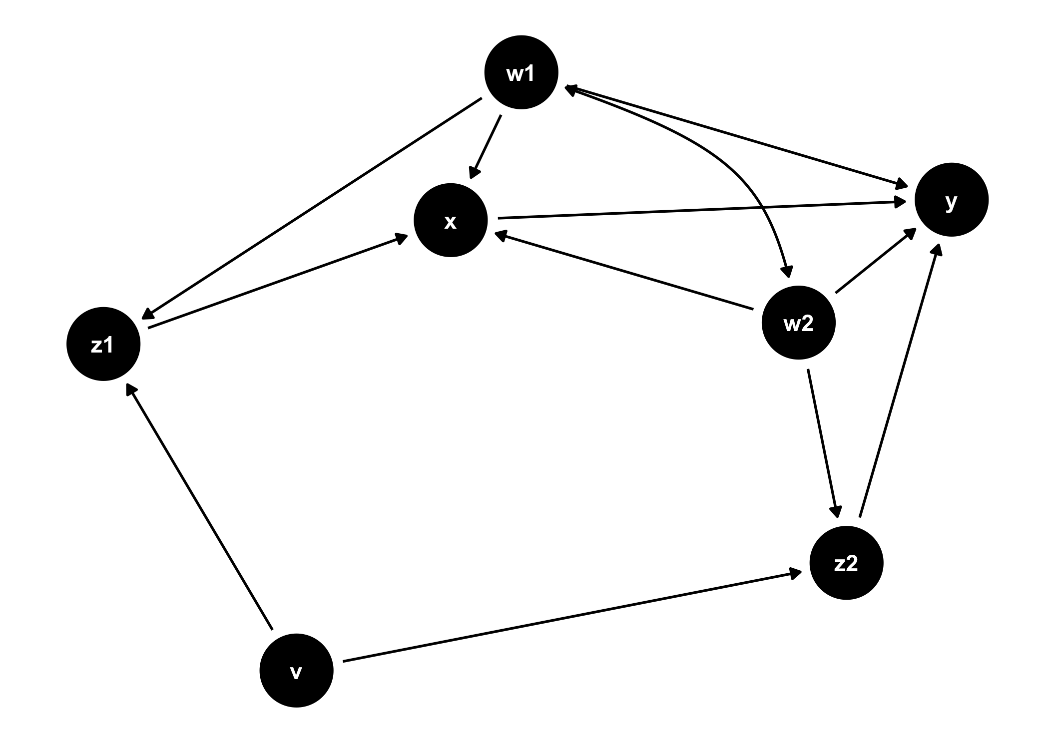
ggdag_adjustment_set(tidy_ggdag, node_size = 14) +
  theme(legend.position = "bottom")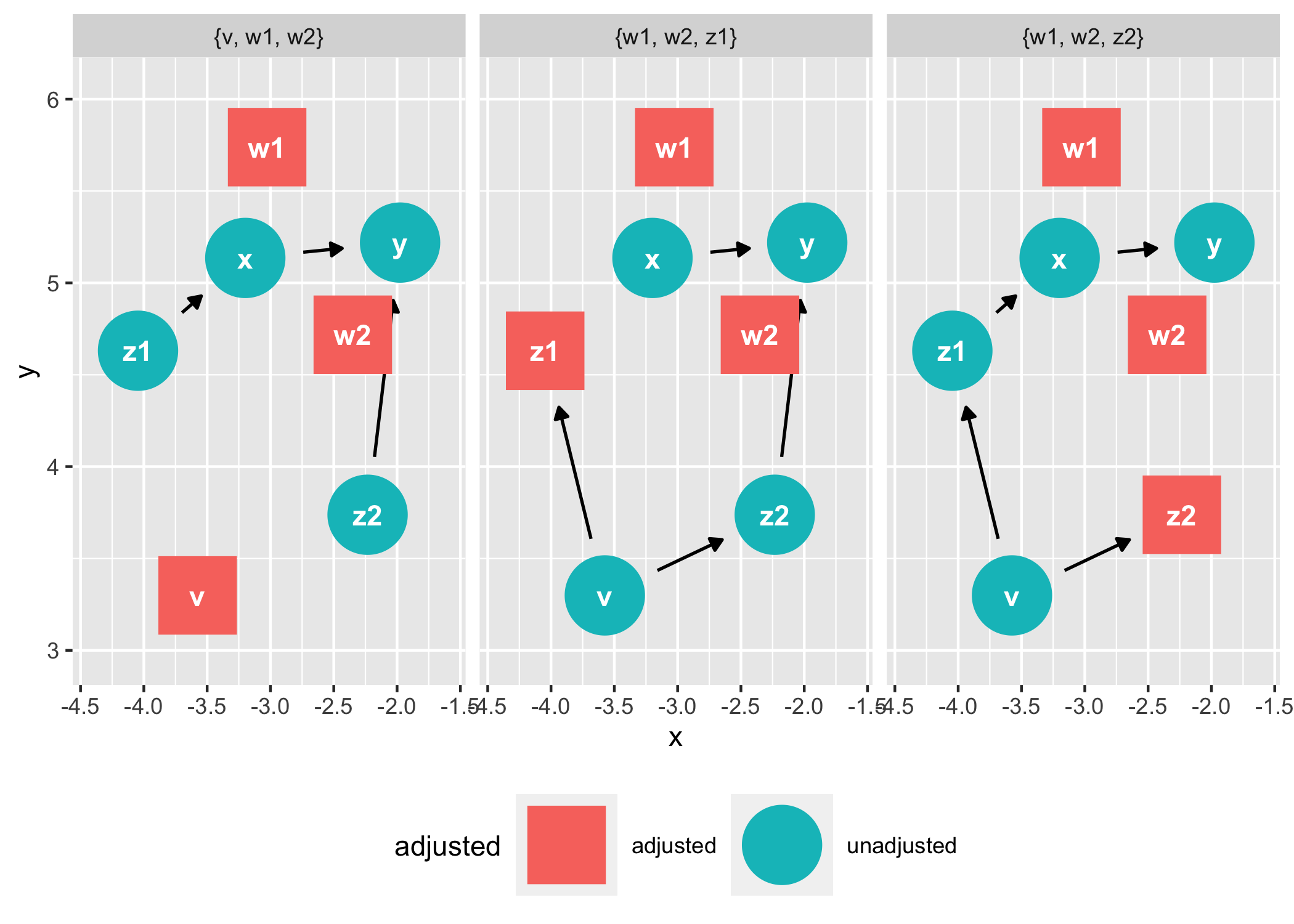
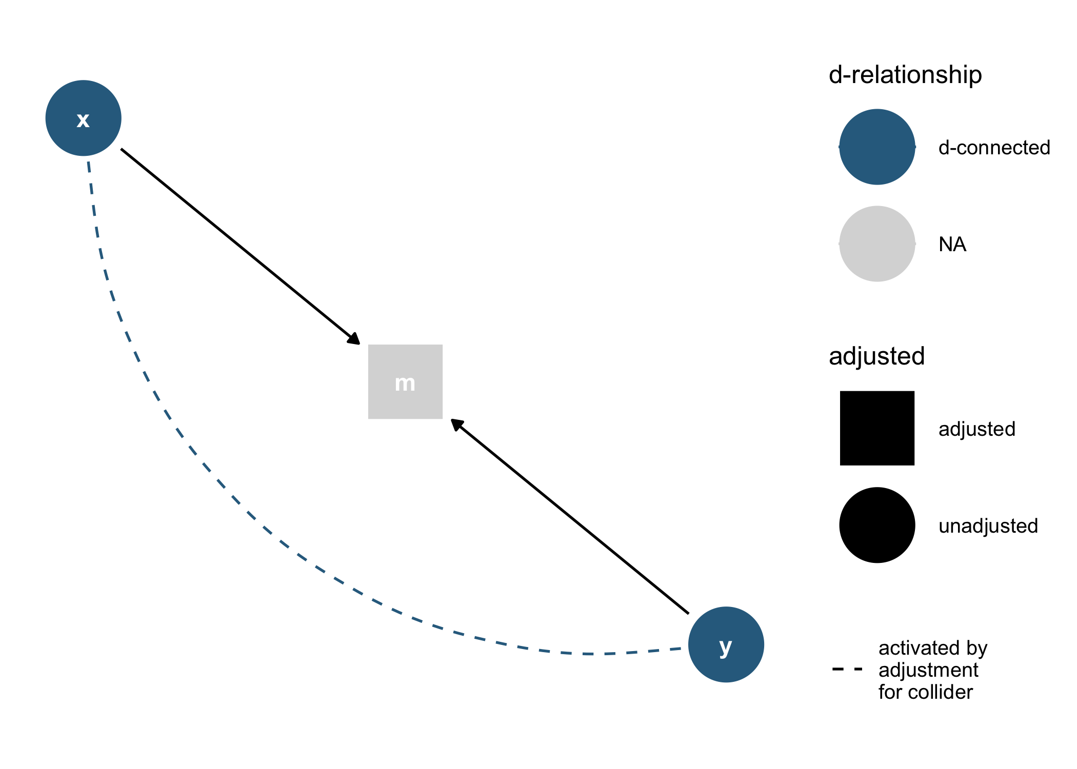
As well as geoms and other functions for plotting them directly in
ggplot2:
dagify(m ~ x + y) %>%
  tidy_dagitty() %>%
  node_dconnected("x", "y", controlling_for = "m") %>%
  ggplot(aes(
    x = x,
    y = y,
    xend = xend,
    yend = yend,
    shape = adjusted,
    col = d_relationship
  )) +
  geom_dag_edges(end_cap = ggraph::circle(10, "mm")) +
  geom_dag_collider_edges() +
  geom_dag_point() +
  geom_dag_text(col = "white") +
  theme_dag() +
  scale_adjusted() +
  expand_plot(expand_y = expansion(c(0.2, 0.2))) +
  scale_color_viridis_d(
    name = "d-relationship",
    na.value = "grey85",
    begin = .35
  )
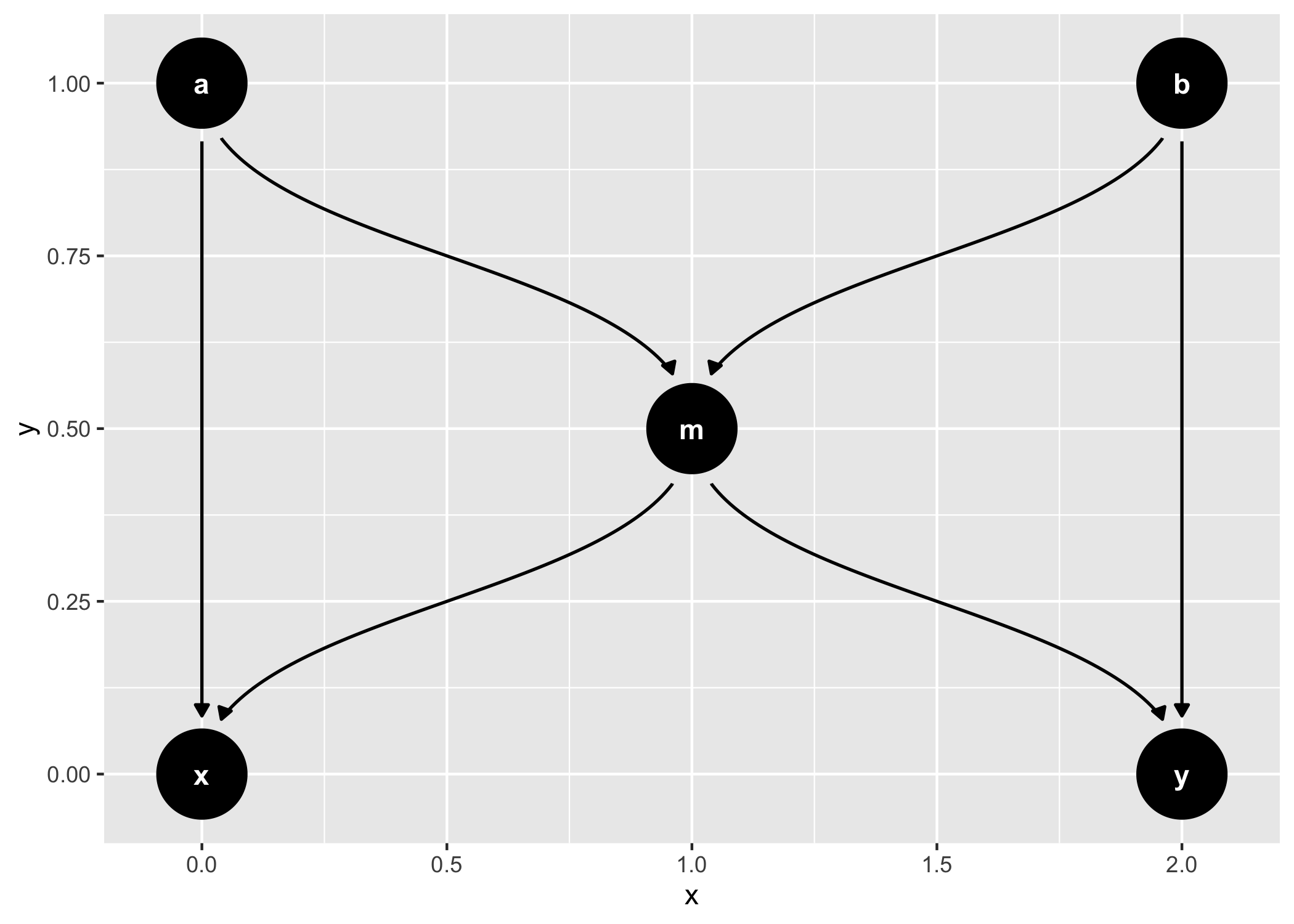
And common structures of bias:
ggdag_equivalent_dags(confounder_triangle())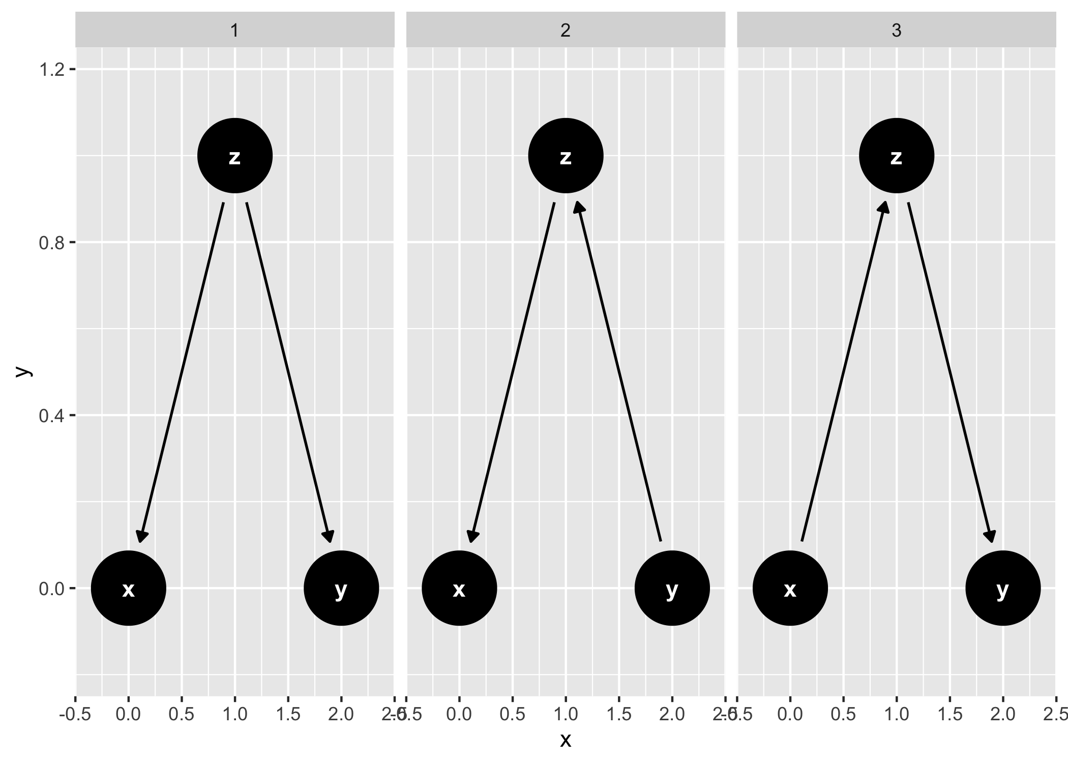
ggdag_butterfly_bias(edge_type = "diagonal")