
ggcube lets you build 3D figures using ggplot2. Use
it to create 3D surfaces, volumes, scatter plots, and complex layered
visualizations using familiar ggplot2 syntax with
aes(x, y, z) and coord_3d().
The package provides a variety of 3D-specific geoms to
render surfaces, prisms, points, paths, and text in 3D; it also works
with some standard ggplot2 layer functions. You can control plot
geometry with 3D projection parameters, apply a range of 3D lighting
models, and mix 3D layers with 2D layers rendered on cube faces.
Standard ggplot2 features like faceting, themes, scales, and legends
work as expected.
3D plots are wonderful for exploration, storytelling, and data art. But note that for precise quantitative communication, where occlusion and perspective distortion can be problematic, 2D is usually the better choice.
# You can install the package from CRAN:
install.packages("ggcube")

# Or get the development version from GitHub:
devtools::install_github("matthewkling/ggcube")R has several other tools for 3D visualization. ggcube is designed for users who want to stay within the ggplot2 ecosystem. Other packages offer different tradeoffs:
The essential ingredient of a ggcube plot is coord_3d().
Adding this to a standard ggplot, and providing a z
aesthetic variable, creates a 3D plot:
library(ggplot2)
library(ggcube)

# Basic 3D scatter plot
ggplot(mpg, aes(x = displ, y = hwy, z = drv, color = class)) +
      geom_point() +
      coord_3d()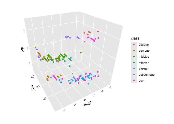
You can control plot rotation, perspective, and dimensions, as well
as axis label placement and panel selection, via parameters to
coord_3d(). See the 3D
view article for a comprehensive guide.
ggplot(mpg, aes(displ, hwy, drv, color = class)) +
      geom_point() +
      coord_3d(pitch = 0, roll = 60, yaw = 0, dist = 1.4,
               ratio = c(2, 1, 1), panels = "all") +
      theme(panel.border = element_rect(color = "black"),
            panel.foreground = element_rect(alpha = .1))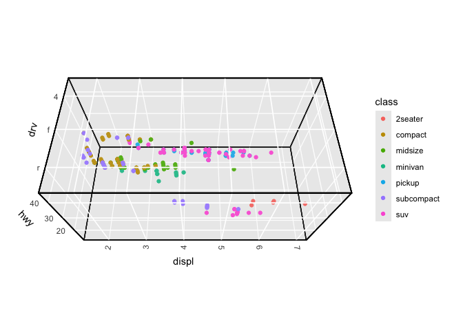
geom_surface_3d() renders surfaces based on existing
grid data such as terrain datageom_ridgeline_3d() renders surfaces as a series of
cross-sectionsgeom_contour_3d() renders surfaces as layer cakes of
stacked contoursstat_function() visualizes mathematical functionsstat_smooth_3d() fits statistical models with two
predictors and visualizes fitted surfaces with confidence intervalsstat_density_3d() creates perspective visualizations of
2D kernel density estimatesstat_hull_3d() plots triangulated volumes based on
convex or alpha hulls of 3D pointsSee the surfaces article for a full guide to surface options.
Example: a terrain surface using geom_surface_3d():
ggplot(mountain, aes(x, y, z)) +
      geom_surface_3d(aes(fill = z, color = z)) +
      scale_fill_viridis_c() + scale_color_viridis_c() +
      coord_3d(ratio = c(1.5, 2, 1), expand = FALSE, panels = "zmin",
               light = light(direction = c(1, 0, 0))) +
      guides(fill = guide_colorbar_3d()) +
      theme_light()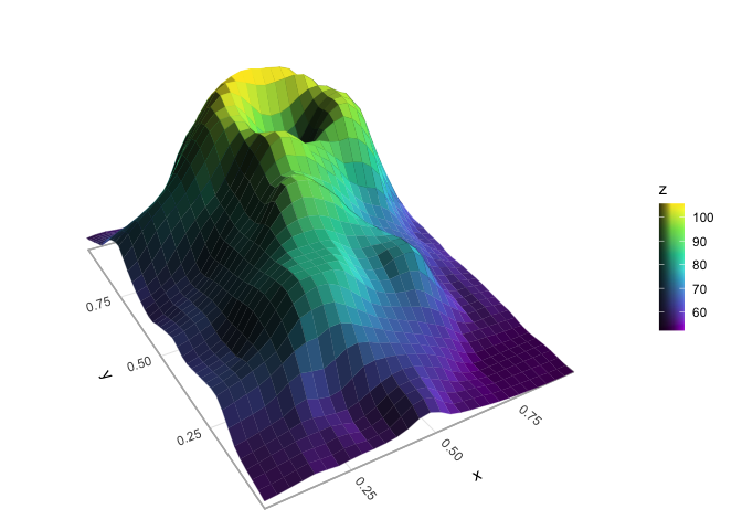
Example: a terrain surface using geom_contour_3d():
ggplot(mountain, aes(x, y, z)) +
      geom_contour_3d(fill = "black", color = "white", linewidth = .5) +
      coord_3d(yaw = 60, ratio = c(1.5, 2, 1), light = "none") +
      theme_void()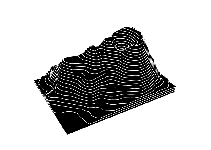
Example: a mathematical surface using
geom_function_3d():
ggplot() +
      geom_function_3d(fun = function(x1, x2) cos(x1) * sin(x2),
                       xlim = c(-pi, pi), ylim = c(-2*pi, 2*pi),
                       fill = "#7a2100", color = "#b3725b",
                       grid = "right1", linewidth = .2) +
      coord_3d(yaw = 160, roll = -70,
               scales = "fixed", ratio = c(1, 1, 2)) +
      labs(x = expression(x[1]),
           y = expression(x[2]),
           z = expression(cos(x[1]) %*% sin(x[2]))) +
      theme_minimal()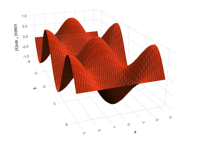
Example: a fitted model surface using
geom_smooth_3d():
# Generate scattered 3D data
set.seed(123)
d <- data.frame(x = rnorm(50),
                y = rnorm(50))
d$z <- d$x + d$x^2 - d$y^2 + rnorm(50)

# Plot GAM fit with uncertainty layers
ggplot(d, aes(x, y, z)) +
      geom_smooth_3d(aes(fill = after_stat(level)),
                     method = "gam", formula = z ~ te(x, y),
                     se = TRUE, level = 0.99,
                     color = "black", grid = "equilateral") +
      scale_fill_manual(values = c("red", "darkorchid4", "steelblue")) +
      coord_3d(light = NULL)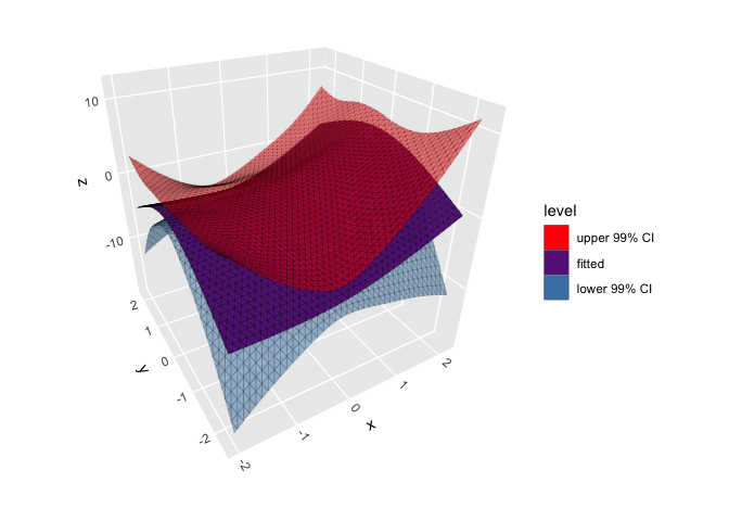
geom_path_3d() renders paths in 3D space with
depth-based sorting and scaling:
butterfly <- ggcube:::lorenz_attractor(n_points = 8000, dt = .01)
ggplot(butterfly, aes(x, y, z, color = time)) +
      geom_path_3d(linewidth = 0.1, color = "black",
                   position = position_on_face(c("xmax", "ymax", "zmin"))) +
      geom_path_3d(linewidth = 0.3) +
      scale_color_gradientn(colors = c("blue", "purple", "red", "orange")) +
      coord_3d() +
      theme_light()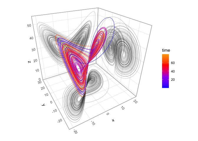
While ggplot2::geom_point() works with ggcube as
demonstrated above, geom_point_3d() creates 3D-aware
scatter plots with proper point ordering, depth-scaled point sizes, and
options to include reference lines and reference points projecting 3D
points onto 2D face panels:
ggplot(mpg, aes(x = displ, y = hwy, z = drv, fill = class)) +
      geom_point_3d(size = 3, shape = 21, color = "black", stroke = .1,
                    ref_lines = TRUE, ref_points = TRUE,
                    ref_faces = c("ymax", "xmax")) +
      coord_3d()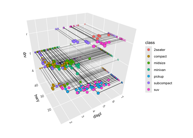
geom_col_3d() produces 3D column chartsgeom_bar_3d() creates 3D histograms of 2D discrete or
continuous variablesgeom_voxel_3d() renders sparse 3D pixel data as arrays
of cubesExample: a 3D histogram using geom_bar_3d():
ggplot(faithful, aes(waiting, eruptions)) +
      geom_bar_3d(fill = "steelblue", color = "steelblue",
                  bins = 15, width = .9) +
      coord_3d(yaw = 60) +
      scale_z_continuous(expand = c(0, 0))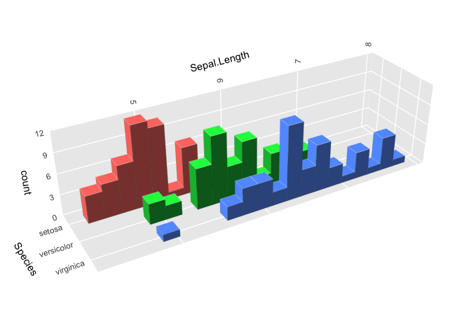
geom_text_3d() creates 3D-aware text, rendered either as
“billboard” text that faces the viewing plane or as 3D polygons that can
face any direction:
df <- expand.grid(x = c("B", "H", "N"), y = c("a", "o", "u"), z = c("g", "t"))
df$label <- paste0(df$x, df$y, df$z)
ggplot(df, aes(x, y, z, label = label, fill = x)) +
      geom_text_3d(method = "polygon", facing = "zmax",
                   size = 5, weight = "bold") +
      coord_3d(scales = "fixed", rotate_labels = FALSE) +
      theme(axis.title = element_blank())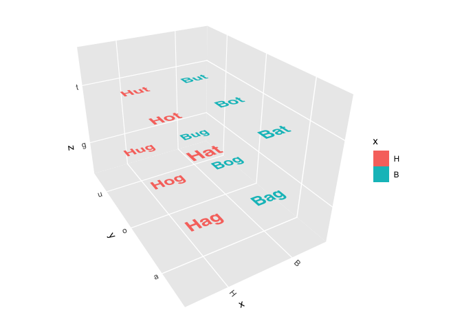
Lighting of 3D polygon layers is controlled by adding a
light() specification to the plot, or providing to the
light parameter of a layer function or
coord_3d(). See the lighting
and shading article for a comprehensive guide.
ggplot(sphere_points, aes(x, y, z)) +
      coord_3d(scales = "fixed") +
      scale_fill_viridis_c() +
      scale_color_viridis_c() +
      theme_dark() +
      theme(legend.position = "none") +

      # apply shading to solid color/fill
      geom_hull_3d(fill = "#8a2900", color = "#8a2900",
                   light = light(method = "direct", mode = "hsl",
                                 direction = c(0, 0, 1))) +

      # apply shading to aesthetic color/fill
      geom_hull_3d(aes(x = x + 2.5, fill = x, color = x),
                   light = light(method = "diffuse", mode = "hsv",
                                 direction = c(0, 0, 1), contrast = 2)) +

      # map surface orientation to 3D RGB color channels
      geom_hull_3d(aes(x = x + 5),
                   light = light(method = "rgb", direction = c(1, 0, -1)))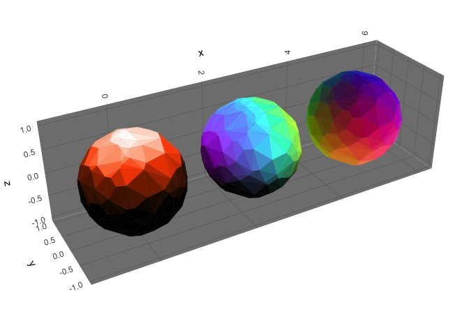
A major limitation of 3D figures is that you can’t get a full view of
the data from any single angle. One way to mitigate this is by rotating
the figure to view the data from different directions. ggcube offers
animated rotation via animate_3d(), and interactive
drag-to-rotate plots via orbit_3d(). See the animation
and interaction article for details. Here’s an example of a rotating
gif:
mammoth <- data.frame(do.call(rbind, rjson::fromJSON(
  file = paste0("https://raw.githubusercontent.com/PAIR-code/",
                "understanding-umap/master/raw_data/mammoth_3d_50k.json")
)))
colnames(mammoth) <- c("Y", "X", "Z")

p <- ggplot(mammoth, aes(X, Y, Z)) +
      geom_hull_3d(method = "alpha", radius = 8,
                   fill = "darkred", color = "darkred") +
      light(mode = "hsl", direction = c(-1, 1, 0), anchor = "camera") +
      coord_3d(roll = -90, scales = "fixed",
               panels = "zmin", expand = FALSE) +
      theme(axis.text = element_blank(),
            axis.ticks = element_blank(),
            axis.title = element_blank())

animate_3d(p, yaw = c(0, 360), nframes = 72, fps = 8, width = 700, cores = 8)
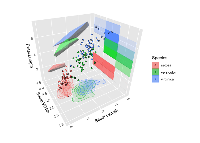
3D and 2D layers can be mixed by using
position_on_face() to project data onto 2D cube faces. We
saw this in the geom_path_3d() example above, but here’s
another example that mixes different geoms, including natively-2D layers
like ggplot2::stat_density_2d():
ggplot(iris, aes(Sepal.Length, Sepal.Width, Petal.Length,
                 color = Species, fill = Species)) +
      coord_3d() + xlim(4, 8) +

      # place 2D density plot on zmin face
      stat_density_2d(position = position_on_face(faces = "zmin", axes = c("x", "y")),
                      geom = "polygon", alpha = .1, linewidth = .25) +

      # flatten 3D hull layer onto ymax face
      geom_hull_3d(position = position_on_face("ymax"), alpha = .5) +

      # flatten 3D voxels onto xmax face to create 2D bins
      geom_voxel_3d(aes(round(Sepal.Length), round(Sepal.Width), round(Petal.Length)),
                    position = position_on_face("xmax"), alpha = .15, light = NULL) +

      # 3D scatter plot (added last so it renders in front)
      geom_point_3d( shape = 21, color = "black", stroke = .25)