


One interface. 50 changepoint methods. Every result tidy, every result plottable.
R has excellent changepoint packages, but each one takes its own
input, returns its own result object, and has its own idea of a plot, so
switching methods means rewriting your analysis. ggchangepoint puts them
behind one interface: cpt_detect() runs any of 50 detection
methods, every result comes back as the same tidy ggcpt
object, and autoplot() draws it, with confidence intervals,
significance regions, posteriors, detector statistics, penalty paths and
accuracy metrics when you need them. When the detector you want is not
one of the 50 (because it is not on CRAN, or lives in Python, or is your
own), cpt_register_method() brings it into the same
grammar.
Install the released version from CRAN:
install.packages("ggchangepoint")Or the development version from GitHub:
# install.packages("devtools")
devtools::install_github("PursuitOfDataScience/ggchangepoint")library(ggchangepoint)
library(ggplot2)Generate a series with a mean shift:
set.seed(2022)
x <- c(rnorm(100, 0, 1), rnorm(100, 10, 1))
Detect changepoints with the unified cpt_detect():
res <- cpt_detect(x, method = "pelt", change_in = "mean")
res
#> ggcpt (changepoint detection result)
#>   Method:             pelt
#>   Change in:          mean
#>   Changepoints found: 1
#>   CP convention:      left
#>   Penalty:            MBIC
#>   Series length:      200
#>
#> Changepoints:
#> # A tibble: 1 × 2
#>      cp cp_value
#>   <int>    <dbl>
#> 1   100    0.467
The result is a ggcpt S3 object, so the broom verbs work
on it: tidy() gives one row per changepoint,
glance() a one-row model summary, and
augment() the original series with segment labels, fitted
values and residuals.
tidy(res)
#> # A tibble: 1 × 2
#>      cp cp_value
#>   <int>    <dbl>
#> 1   100    0.467
glance(res)
#> # A tibble: 1 × 9
#>       n n_changepoints method change_in penalty_type penalty_value cp_convention
#>   <int>          <int> <chr>  <chr>     <chr>                <dbl> <chr>
#> 1   200              1 pelt   mean      MBIC                    NA left
#> # ℹ 2 more variables: total_cost <dbl>, runtime <dbl>
Visualise with autoplot():
autoplot(res)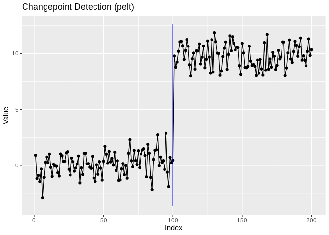
cpt_detect(x, method = "...") dispatches to 50 methods,
from classic PELT to Bayesian online detection, functional data and
dynamic networks.ggcpt object, with tidy(),
glance(), and augment(), and a time index that
survives the round trip.autoplot() draws any
result: changepoints, confidence intervals, significance regions, fitted
signals, posteriors, multivariate facets, and (type =) the
detector’s own statistic, solution path or scale space.as_ggcpt() and
cpt_register_method() bring any external detector into the
same tidy, plottable grammar.| Family | Methods |
|---|---|
| Penalised / optimal partitioning | PELT · BinSeg · SegNeigh · AMOC · FPOP · binsegRcpp (fast) · CPOP (slope) · fastcpd (mean/var/AR/ARMA/GARCH) |
| Multiscale / search | WBS · WBS2 · TGUH · NOT · MOSUM · Isolate-Detect · SMUCE · HSMUCE (the last two with CIs) · WBSTS (nonstationary) |
| Inference | NSP: significance regions, each guaranteed to contain a change at a global level |
| Nonparametric / kernel | ED-PELT · E-Divisive / E-Agglo · kernel running stats · NP-MOJO · sequential CPM · self-normalisation · KWC depth ranks |
| Bayesian | bcp posteriors · online BOCPD · BEAST model averaging · mcp (formula-based, full posteriors) |
| High-dimensional | inspect · ocd · geomcp · ESAC · Pilliat · high-dimensional covariance · VAR(1) · high-dimensional regression |
| Functional & network | functional mean · functional covariance · KWC · fabisearch (NMF
network structure) · changepoints networks |
| Regression, trend & season | Bai-Perron · segmented · EnvCpt · DeCAFS · BFAST (season + trend) |
| Classical single-change tests | Pettitt · Buishand · SNHT · Taylor’s analyzer |
Run cpt_methods() for the live table with engines,
installation status and capability flags. Only three engines are
required (changepoint, changepoint.np and
ecp); every other engine lives in Suggests and
is loaded on demand, so a plain install stays light.
cpt_install_engines("bayesian") installs a whole family at
once.
cpt_detect() dispatches to any supported method by
name:
cpt_detect(x, method = "binseg", change_in = "mean")
#> ggcpt (changepoint detection result)
#>   Method:             binseg
#>   Change in:          mean
#>   Changepoints found: 1
#>   CP convention:      left
#>   Penalty:            MBIC
#>   Series length:      200
#>
#> Changepoints:
#> # A tibble: 1 × 2
#>      cp cp_value
#>   <int>    <dbl>
#> 1   100    0.467
cpt_detect(x, method = "wbs", change_in = "mean")
#> ggcpt (changepoint detection result)
#>   Method:             wbs
#>   Change in:          mean
#>   Changepoints found: 1
#>   CP convention:      left
#>   Penalty:            sSIC
#>   Series length:      200
#>
#> Changepoints:
#> # A tibble: 1 × 2
#>      cp cp_value
#>   <int>    <dbl>
#> 1   100    0.467
cpt_detect(x, method = "fpop", change_in = "mean")
#> ggcpt (changepoint detection result)
#>   Method:             fpop
#>   Change in:          mean
#>   Changepoints found: 1
#>   CP convention:      left
#>   Penalty:            Manual = 17.846
#>   Series length:      200
#>
#> Changepoints:
#> # A tibble: 1 × 2
#>      cp cp_value
#>   <int>    <dbl>
#> 1   100    0.467
Use cpt_methods() to see all available and planned
methods with their engine packages and installation status:
cpt_methods()
#> # A tibble: 55 × 15
#>    method   change_in        engine status installed target_release multivariate
#>    <chr>    <chr>            <chr>  <chr>  <lgl>     <chr>          <lgl>
#>  1 pelt     mean, var, mean… chang… avail… TRUE      <NA>           FALSE
#>  2 binseg   mean, var, mean… chang… avail… TRUE      <NA>           FALSE
#>  3 segneigh mean, var, mean… chang… avail… TRUE      <NA>           FALSE
#>  4 amoc     mean, var, mean… chang… avail… TRUE      <NA>           FALSE
#>  5 np       distribution     chang… avail… TRUE      <NA>           FALSE
#>  6 ecp      distribution (m… ecp    avail… TRUE      <NA>           TRUE
#>  7 fpop     mean             fpop   avail… TRUE      <NA>           FALSE
#>  8 wbs      mean             wbs    avail… TRUE      <NA>           FALSE
#>  9 wbs2     mean             break… avail… TRUE      <NA>           FALSE
#> 10 not      mean, var, mean… not    avail… TRUE      <NA>           FALSE
#> # ℹ 45 more rows
#> # ℹ 8 more variables: univariate <lgl>, online <lgl>, ci <lgl>, fitted <lgl>,
#> # posterior <lgl>, statistic <lgl>, path <lgl>, scale_space <lgl>Real series have dates, and “changepoint at index 147” is a
translation step the analyst should not have to do. Pass an
index (or a ts, xts,
zoo or tsibble) and detection still runs on
positions (every engine assumes an equally spaced sequence) while
everything reported comes back on your scale:
dates <- as.Date("2020-01-01") + seq_along(x) - 1
dated <- cpt_detect(x, method = "pelt", index = dates)
tidy(dated)
#> # A tibble: 1 × 3
#>      cp cp_index   cp_value
#>   <int> <date>        <dbl>
#> 1   100 2020-04-09    0.467
autoplot(dated)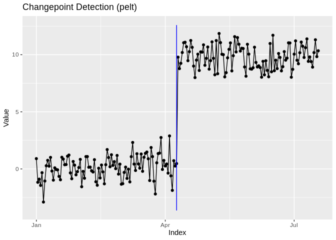
as_cpt_series() is the same conversion on its own, for
code that needs the values and the index before detection runs.
There is a data-frame interface too, taking a bare column name, a string, or a position:
df <- data.frame(day = dates, value = x)
cpt_detect(df, y = value, index = day, method = "pelt")
#> ggcpt (changepoint detection result)
#>   Method:             pelt
#>   Change in:          mean
#>   Changepoints found: 1
#>   CP convention:      left
#>   Penalty:            MBIC
#>   Series length:      200
#>   Index:              2020-01-01 to 2020-07-18
#>
#> Changepoints:
#> # A tibble: 1 × 3
#>      cp cp_index   cp_value
#>   <int> <date>        <dbl>
#> 1 100 2020-04-09 0.467SMUCE (smuce_wrapper(), via stepR) delivers
a confidence interval for every changepoint location; Bai-Perron
(strucchange_wrapper()) and broken-line regression
(segmented_wrapper()) do the same for regression breaks.
The intervals live in ci_lower/ci_upper
columns and render with autoplot(show_ci = TRUE) or the
geom_cpt_ci() layer:
res_smuce <- smuce_wrapper(x)
tidy(res_smuce)
#> # A tibble: 2 × 4
#>      cp cp_value ci_lower ci_upper
#>   <int>    <dbl>    <int>    <int>
#> 1     7   -1.06         2       94
#> 2   100    0.467      100      100
autoplot(res_smuce, show_ci = TRUE, show_fit = TRUE)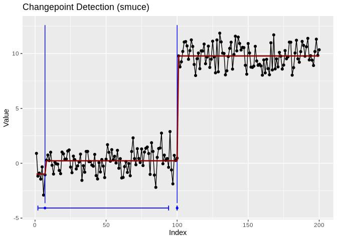
Read the intervals, not just the locations: the genuine shift is pinned to a single index, while the spurious early changepoint carries an interval nearly a hundred observations wide, exactly the distinction a bare list of locations hides.
Bayesian engines return posterior probabilities instead:
bcp_wrapper() (posterior probability of a change at every
location), beast_wrapper() (Bayesian model averaging), and
bocpd_wrapper() (online run-length posterior). Two
dedicated displays accompany them, ggcpt_posterior() and
ggcpt_runlength():
res_bcp <- bcp_wrapper(x, seed = 1)
tidy(res_bcp)
#> # A tibble: 1 × 3
#>      cp cp_value posterior_prob
#>   <int>    <dbl>          <dbl>
#> 1   100    0.467              1
ggcpt_posterior(res_bcp)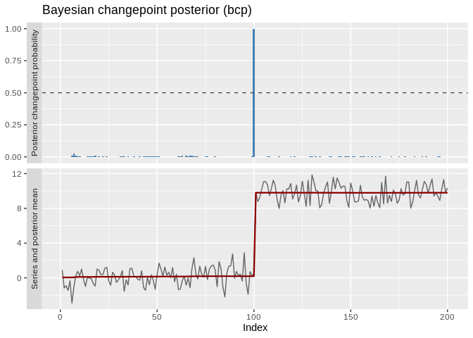
Instead of guessing one penalty, cpt_crops() computes
every optimal segmentation over a penalty range
(Haynes, Eckley and Fearnhead, 2017) and plots the elbow diagnostic, the
penalty path, or the candidate segmentations themselves:
set.seed(2021)  # local, so this example does not depend on the chunks above
path <- cpt_crops(c(rnorm(100), rnorm(100, 3), rnorm(100, -1)))
path
#> ggcpt_path (CROPS penalty path)
#>   Change in:              mean
#>   Penalty range:          [5.704, 57.04]
#>   Series length:          300
#>   Distinct segmentations: 4
#>
#> # A tibble: 4 × 3
#>   penalty n_cpts  cost
#>     <dbl>  <int> <dbl>
#> 1    8.44      2  320.
#> 2    8.08      4  303.
#> 3    6.91      5  295.
#> 4    5.70      7  281.
autoplot(path)                          # cost elbow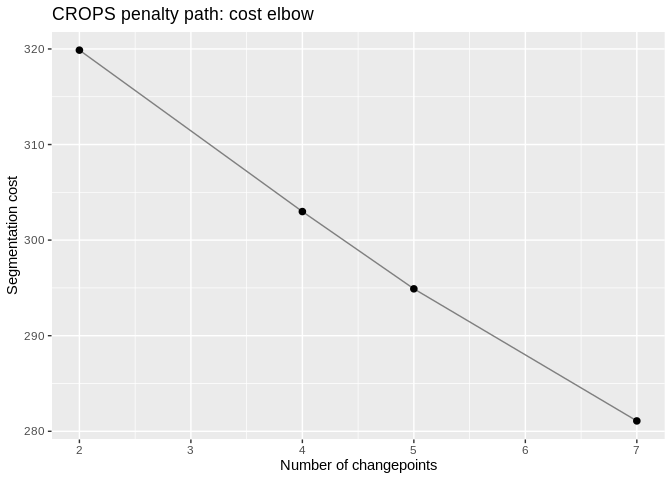
autoplot(path, type = "segmentations") # see the actual candidate models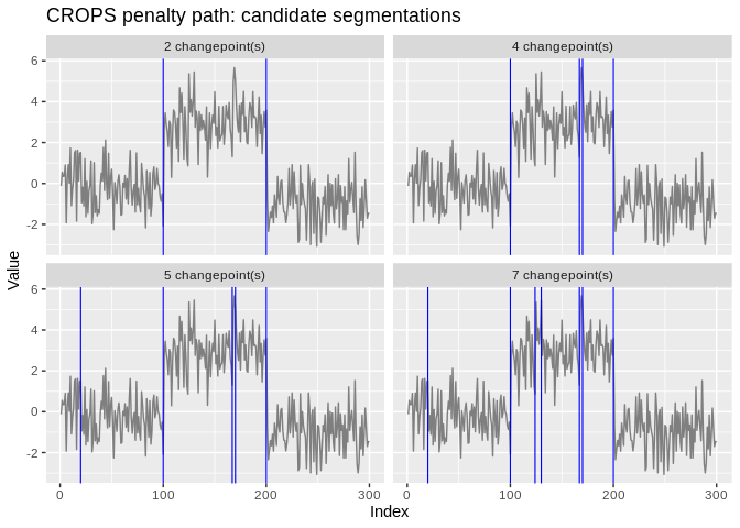
Narrowest Significance Pursuit (Fryzlewicz 2024) inverts the usual framing: instead of estimating locations and then asking whether they are real, it returns intervals, each guaranteed to contain at least one changepoint, with the guarantee holding globally across all of them. That is a different visual object, and it gets its own layer:
res_nsp <- nsp_wrapper(x, M = 100, seed = 1)
cpt_regions(res_nsp)
#> # A tibble: 1 × 4
#>   start   end length value
#>   <int> <int>  <int> <dbl>
#> 1   100   101      2  4.66
autoplot(res_nsp)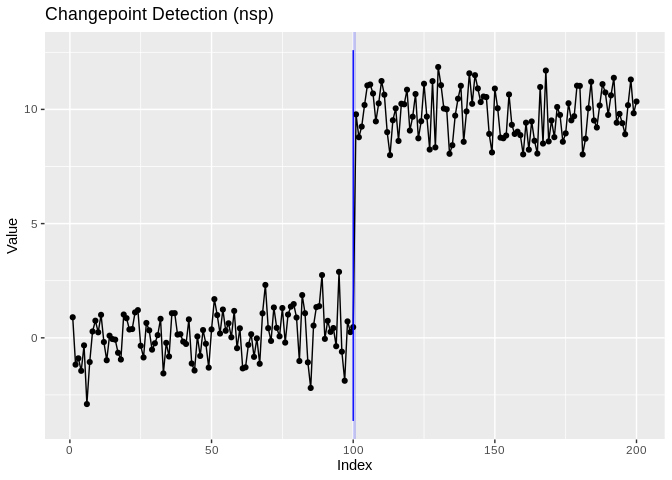
The cp column of an NSP fit is the interval midpoint, is
labelled as such in cp_source, and is never presented as an
estimate: the region is the inferential object.
For every other engine, cpt_confint() answers “where
could this changepoint be?” behind one contract, and says which of four
routes it used:
cpt_confint(res, method = "bootstrap", B = 50, seed = 1)
#> # A tibble: 1 × 6
#>      cp ci_lower ci_upper level source    n_replicates
#>   <int>    <int>    <int> <dbl> <chr>            <int>
#> 1   100      100      100  0.95 bootstrap           50
cpt_test() attaches a test to each changepoint, using
the engine’s own where it has one and an explicitly unadjusted
two-sample test where it does not, with a
selection_adjusted column recording whether the p-value
accounts for the fact that the location was chosen by looking
at the data, which only one of the engine tests does:
suppressWarnings(cpt_test(res))
#> # A tibble: 1 × 6
#>      cp estimate statistic   p_value method                   selection_adjusted
#>   <int>    <dbl>     <dbl>     <dbl> <chr>                    <lgl>
#> 1 100 9.66 67.1 4.48e-138 Welch two-sample t (una… FALSEcpt_crops() draws the penalty path;
cpt_select() actually chooses, by BIC, the
Zhang-Siegmund segment-length mBIC, AIC, an explicit knee rule on the
CROPS curve, order-preserved cross-validation (the criterion with a
consistency proof), or bootstrap stability:
set.seed(2022)  # local, so this example does not depend on the chunks above
x3 <- c(rnorm(120), rnorm(120, 4), rnorm(120, 1))
sel <- cpt_select(x3, criterion = "mbic", k_max = 6)
sel
#> ggcpt_selection (criterion: mbic, method: pelt)
#>   Candidates scored: K = 0 to 6
#>   Chosen K:          2
#>   Locations:         120, 240
#>
#> # A tibble: 7 × 4
#>       k value  cost chosen
#>   <int> <dbl> <dbl> <lgl>
#> 1     0 457.  457.  FALSE
#> 2     1 337.  320.  FALSE
#> 3     2  14.2 -17.9 TRUE
#> 4     3  18.5 -27.2 FALSE
#> 5     4  27.3 -32.5 FALSE
#> 6     5  37.7 -37.2 FALSE
#> 7     6  42.9 -46.5 FALSE
autoplot(sel, plot_type = "ladder", max_facets = 5)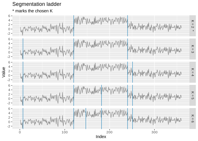
Every detector computes something (a MOSUM statistic at each bandwidth, a set of random intervals with contrast values, a nested sequence of splits), and keeping only the argmax throws away the explanation. Three accessors give it back:
set.seed(2023)  # local, so this example does not depend on the chunks above
res_mosum <- cpt_detect(c(rnorm(200), rnorm(200, 3)), method = "mosum")
autoplot(res_mosum, type = "statistic")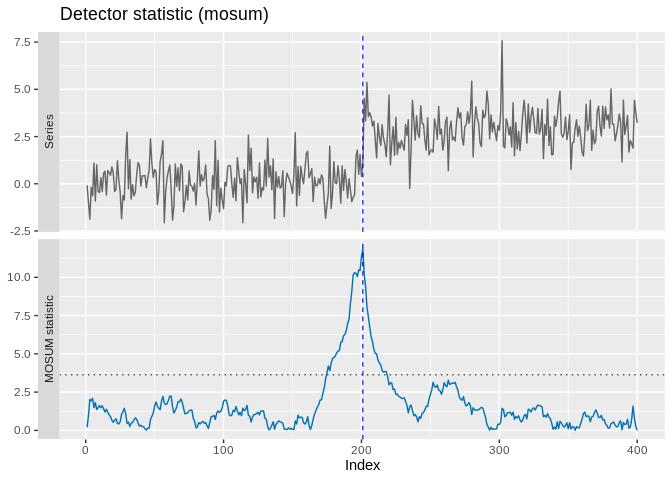
ggcpt_scale_space(res_mosum, bandwidths = c(20, 40, 80))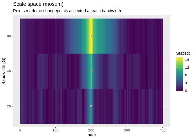
cpt_statistic() returns the profile as a tibble and
ggcpt_statistic() draws it on its own;
cpt_solution_path() and ggcpt_solution_path()
do the same for the order in which candidates entered a
binary-segmentation or wild-binary-segmentation model.
cpt_stability() answers “would I find this again?”.
cpt_influence() answers the sharper question, perturbing
one observation at a time and re-fitting, with the
Wilms-Killick-Matteson diagnostic family rendered in ggplot2:
inf <- cpt_influence(res, engine = "recompute", subset = seq(1, 200, by = 5))
head(cpt_leverage(inf), 3)
#> # A tibble: 3 × 5
#>   index delta_n_cp max_shift param_shift leverage
#>   <int>      <int>     <dbl>       <dbl>    <dbl>
#> 1     6          0         0      0.0307     3.74
#> 2   141          0         0      0.0180     1.66
#> 3   181          0         0      0.0179     1.64
autoplot(inf)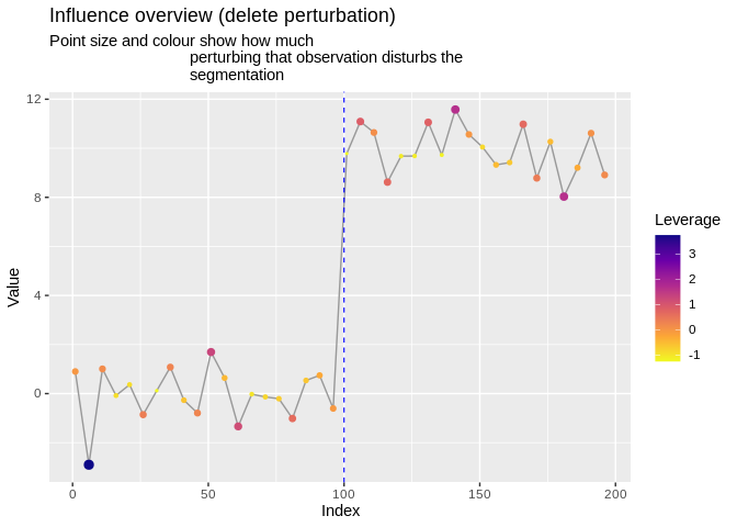
cpt_sensitivity() is the tuning-parameter analogue, and
the direct answer to “is this robust to the penalty?”:
autoplot(cpt_sensitivity(x3, method = "pelt", over = list(penalty = c(4, 20, 80))))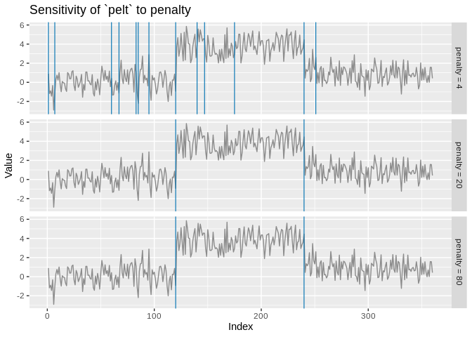
An expert marks intervals as containing a change or not, accuracy is measured in label errors, and the penalty is learned rather than assumed (Hocking et al., 2013). The central object is a rectangle drawn over a time series, a ggplot2-native idea:
labs <- cpt_labels(c(80, 140), c(120, 190), c("one_change", "no_change"))
ggplot(data.frame(t = seq_along(x), y = x), aes(t, y)) +
  geom_cpt_label(aes(xmin = start, xmax = end, fill = change), data = labs) +
  geom_line() +
  scale_fill_cpt_label() +
  theme_ggcpt()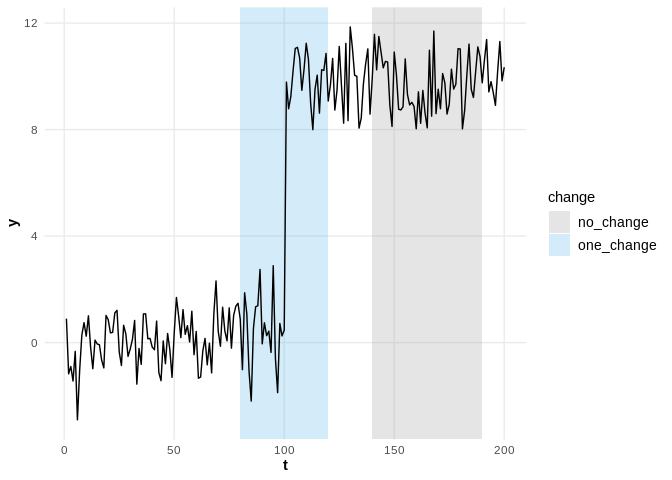
cpt_label_error(res, labs)
#> cpt_label_error (2 label(s))
#>   correct: 2   false positives: 0   false negatives: 0
#>   total label errors: 0
#>
#> # A tibble: 2 × 7
#>   label_id series start   end change     n_changes status
#>      <int> <chr>  <int> <int> <chr>          <int> <chr>
#> 1        1 <NA>      80   120 one_change         1 correct
#> 2        2 <NA>     140   190 no_change          0 correct
cpt_label_error_curve() sweeps the penalty and reports
false positives, false negatives and total label error at each value:
the curve the learned penalty is chosen to minimise.
cpt_learn_penalty() fits the max-margin interval regression
over a set of labelled series, and the model plugs straight into
cpt_detect():
set.seed(2024)  # local, so this example does not depend on the chunks above
series <- list(a = c(rnorm(60), rnorm(60, 4)), b = c(rnorm(80), rnorm(80, 2)))
labels <- list(a = as_cpt_labels(60, n = 120), b = as_cpt_labels(80, n = 160))
model <- cpt_learn_penalty(series, labels, penalties = c(1, 4, 16, 64, 256))
cpt_detect(series$a, method = "pelt", penalty = model)
#> ggcpt (changepoint detection result)
#>   Method:             pelt
#>   Change in:          mean
#>   Changepoints found: 1
#>   CP convention:      left
#>   Penalty:            Manual = 43.469
#>   Series length:      120
#>
#> Changepoints:
#> # A tibble: 1 × 2
#>      cp cp_value
#>   <int>    <dbl>
#> 1 60 -0.0326cpt_recommend() turns the capability matrix into advice,
and is explicit about what each choice assumes:
cpt_recommend(noise = "autocorrelated")
#> Recommended methods for: univariate series, change in mean, autocorrelated noise
#>
#> 1. decafs (DeCAFS)
#>    why: handles change_in = "mean"; built for autocorrelated noise
#> 2. envcpt (EnvCpt)
#>    why: handles change_in = "mean"; built for autocorrelated noise
#> 3. nsp (nsp)
#>    why: handles change_in = "mean"; built for autocorrelated noise
#> 4. sn (SNSeg)
#>    why: handles change_in = "mean"; built for autocorrelated noise
#> 5. wbsts (wbsts)
#>    why: handles change_in = "mean"; built for autocorrelated noise
#>
#> (31 further candidate(s); the full table is the return value.)
#>
#> Cite the method you use with cpt_cite(). Cross-check the choice with
#> cpt_consensus() and cpt_sensitivity().
cpt_consensus() runs several detectors and reports the
locations they agree on, a robustness display, not a significance
test:
cons <- cpt_consensus(x3, methods = c("pelt", "binseg", "wbs", "amoc"))
tidy(cons)
#> # A tibble: 2 × 5
#>      cp cp_value votes methods                 spread
#>   <int>    <dbl> <int> <chr>                    <int>
#> 1   120   -0.927     4 amoc, binseg, pelt, wbs      0
#> 2   240    4.45      3 binseg, pelt, wbs            0
autoplot(cons, plot_type = "agreement")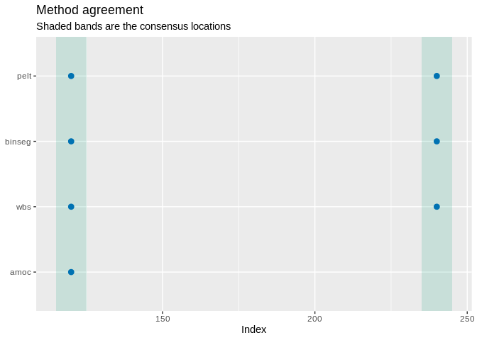
“Changepoint at index 147” is not a finding.
cpt_annotate_events() matches detections to known events
and reports all three outcomes, and the unexplained changepoints are
where the interesting analysis starts:
events <- data.frame(when = as.Date(c("2020-04-09", "2020-06-01")),
                     what = c("policy change", "supply shock"))
cpt_annotate_events(dated, events)
#> ggcpt_events (tolerance 5 position(s))
#>   Changepoints explained by an event: 1
#>   Changepoints with no event:         0
#>   Events with no changepoint:         1
#>
#> Matched:
#> # A tibble: 1 × 6
#>      cp cp_index   event         event_value event_position distance
#>   <int> <date>     <chr>         <date>               <int>    <int>
#> 1   100 2020-04-09 policy change 2020-04-09             100        0
#>
#> Events the detector did not find:
#> # A tibble: 1 × 3
#>   event        event_value event_position
#>   <chr>        <date>               <int>
#> 1 supply shock 2020-06-01             153
cpt_report() assembles the whole analysis (method,
citation, penalty, locations with intervals, segments, the call and
sessionInfo()) into one reproducible artifact, and
cpt_gt() renders a publication-ready table.
cpt_benchmark() runs a method-by-dataset grid, scores
every cell, and records an engine failure instead of losing the run:
bm <- cpt_benchmark(cpt_datasets(n = 300, seed = 1),
                    methods = c("pelt", "binseg", "wbs", "amoc"),
                    progress = FALSE)
bm
#> ggcpt_benchmark (9 dataset(s) x 4 method(s), tolerance 5)
#>
#> Mean rank across datasets (1 = best):
#> # A tibble: 4 × 4
#>   method mean_rank n_datasets n_datasets_total
#>   <chr>      <dbl>      <int>            <int>
#> 1 pelt        2.11          9                9
#> 2 wbs         2.11          9                9
#> 3 binseg      2.5           9                9
#> 4 amoc        3.28          9                9
#>
#> # A tibble: 36 × 4
#>    dataset  method covering    f1
#>    <chr>    <chr>     <dbl> <dbl>
#>  1 blocks   pelt      0.993 1
#>  2 fms      pelt      0.135 0
#>  3 mix      pelt      0.420 0
#>  4 teeth    pelt      1     1
#>  5 stairs   pelt      1     1
#>  6 step     pelt      0.993 1
#>  7 ar1      pelt      1     1
#>  8 heavy    pelt      0.817 0.5
#>  9 varshift pelt      0.552 0
#> 10 blocks   binseg    0.699 0.625
#> 11 fms      binseg    0.135 0
#> 12 mix      binseg    0.422 0
#> # ℹ 24 more rows
autoplot(bm)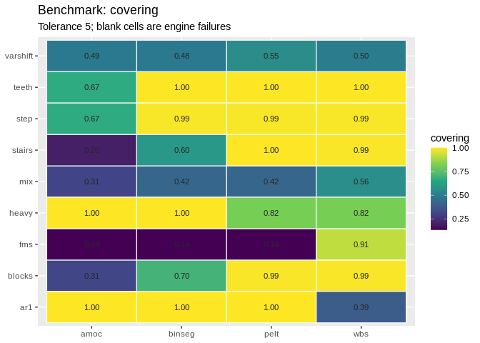
cpt_datasets() is offline and deterministic. For the
real thing, cpt_load_tcpd() downloads and caches the Turing
Change Point Dataset, multi-annotator ground truth intact, and
cpt_annotations() lays that ground truth out one row per
annotator per changepoint.
cpm, ocd and BOCPD are online
methods, and for an online method “did you find the location?” is the
wrong question. cpt_monitor() is a stateful detector you
feed as data arrive; cpt_delay() scores it on detection
delay and false alarms:
set.seed(2025)  # local, so this example does not depend on the chunks above
mon <- cpt_replay(c(rnorm(200), rnorm(200, 3)), method = "edetector")
alarms(mon)
#> # A tibble: 1 × 3
#>    time statistic threshold
#>   <int>     <dbl>     <dbl>
#> 1   101      191.       100
cpt_delay(mon, truth = 200)
#> ggcpt_delay
#>   True changes:       1
#>   Detected:           1
#>   Mean delay:         1
#>   Median delay:       1
#>   False alarms:       0
#>   Average run length: no false alarms
#>
#> # A tibble: 1 × 4
#>   truth alarm delay detected
#>   <int> <int> <dbl> <lgl>
#> 1   200   201     1 TRUE
cpt_replay() is the batch convenience; in production you
build the monitor once with cpt_monitor() and push each new
observation through cpt_update() as it arrives.
"edetector" is a native implementation of the mixture
Shiryaev-Roberts e-detector (Shin, Ramdas and Rinaldo, 2023), the one
method here that is implemented rather than wrapped, because no R
package implements it and it carries a finite-sample average-run-length
guarantee of at least 1 / alpha with no calibration run:
the shift mixture is a uniform average, so M_t - t
is a mean-zero martingale under the null and optional stopping at the
alarm time bounds the in-control run length.
The question that should precede the analysis:
pw <- cpt_power(n = 300, jump = c(0.25, 0.5, 1, 2), n_sim = 50, seed = 1)
pw
#> ggcpt_power (method: pelt, change in mean, gauss noise, tolerance 5)
#>   4 scenario(s), 50 replicates each
#>
#> # A tibble: 4 × 9
#>       n  jump sigma location power  mc_se mean_abs_error false_positives n_sim
#>   <int> <dbl> <dbl>    <int> <dbl>  <dbl>          <dbl>           <dbl> <int>
#> 1   300  0.25     1      150  0    0              NaN               0       50
#> 2   300  0.5      1      150  0.38 0.0686           2.11            0.22    50
#> 3   300  1        1      150  0.72 0.0635           1.83            0.28    50
#> 4   300  2        1      150  1    0                0.38            0       50
#>
#> Monte Carlo standard errors are in `mc_se`; a power of 0.80 from 50
#> replicates is only known to about +/- 0.11.
autoplot(pw)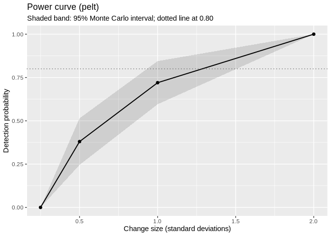
cpt_min_detectable() inverts it and returns the smallest
change reaching a target power, the number that belongs in a
pre-registration. cpt_scenarios() builds the matching grid
of labelled synthetic series, so the same design can be fed straight to
cpt_benchmark().
Not every method is on CRAN, and some of the interesting ones never
will be. cpt_register_method() teaches
cpt_detect() about anything callable from R, and the whole
toolchain follows:
cpt_register_method(
  "biggest_jump",
  fn = function(x, ...) which.max(abs(diff(x))),
  engine = "example",
  citation = "No citation supplied (illustration only)."
)
cpt_detect(x, method = "biggest_jump")
#> ggcpt (changepoint detection result)
#>   Method:             biggest_jump  [user-registered]
#>   Change in:          mean
#>   Changepoints found: 1
#>   CP convention:      left
#>   Penalty:            MBIC
#>   Series length:      200
#>
#> Changepoints:
#> # A tibble: 1 × 2
#>      cp cp_value
#>   <int>    <dbl>
#> 1   100    0.467
#>
#> This result came from a user-registered detector; the package validated
#> its shape, not its statistics. See ?cpt_register_method.
subset(cpt_methods(), status == "registered")
#> # A tibble: 1 × 15
#>   method       change_in engine  status    installed target_release multivariate
#>   <chr>        <chr>     <chr>   <chr>     <lgl>     <chr>          <lgl>
#> 1 biggest_jump mean      example register… NA        <NA>           FALSE
#> # ℹ 8 more variables: univariate <lgl>, online <lgl>, ci <lgl>, fitted <lgl>,
#> #   posterior <lgl>, statistic <lgl>, path <lgl>, scale_space <lgl>
cpt_unregister_method("biggest_jump")
Registered methods are visibly user-supplied:
cpt_registered_methods() lists just those,
cpt_methods() marks them, print() says so on
every result, and cpt_cite() returns the citation you gave
or states plainly that none was given. as_ggcpt() does the
same job for a bare set of changepoints (a published paper’s reported
breaks, say) without registering anything.
ggcpt_compare() runs several detectors on the same
series and facets the results, so agreement (and disagreement) is
visible at a glance:
ggcpt_compare(x, methods = c("pelt", "binseg", "fpop", "wbs"))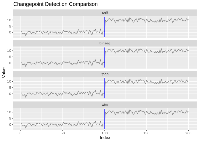
For a numeric summary, use ggcpt_compare_table():
ggcpt_compare_table(x, methods = c("pelt", "binseg", "fpop", "wbs"))
#> # A tibble: 4 × 3
#>   method    cp cp_value
#>   <chr>  <int>    <dbl>
#> 1 pelt     100    0.467
#> 2 binseg   100    0.467
#> 3 fpop     100    0.467
#> 4 wbs 100 0.467cpt_batch() runs one detector over many series (a
matrix, data frame, or list) and returns a tidy tibble of results,
honouring future::plan() for parallel execution.
cpt_stability() bootstrap-resamples within fitted segments
and reports how often each location is re-detected, a cheap confidence
signal for engines with no native intervals:
set.seed(2026)  # local, so this example does not depend on the chunks above
X <- cbind(shifted = x, noise = rnorm(200))
batch <- cpt_batch(X, method = "pelt")
batch
#> ggcpt_batch (2 series, method: pelt)
#>
#> # A tibble: 2 × 2
#>   series  n_changepoints
#>   <chr>            <int>
#> 1 shifted              1
#> 2 noise                0
autoplot(batch)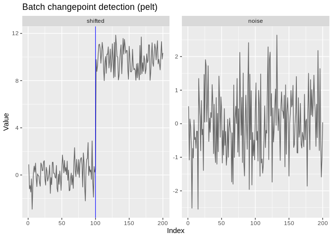
st <- cpt_stability(x, method = "pelt", B = 50, seed = 1)
st
#> ggcpt_stability (50 bootstrap replicates, method: pelt)
#>
#> Original changepoints and their re-detection frequency:
#> # A tibble: 1 × 2
#>      cp stability
#>   <int>     <dbl>
#> 1   100         1
autoplot(st)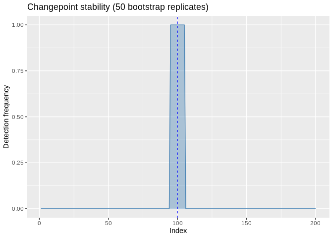
The multivariate engines accept a matrix (rows are time points)
directly through cpt_detect() and render as faceted
small-multiples:
set.seed(1)
Xhd <- cbind(a = c(rnorm(80), rnorm(80, 3)),
             b = c(rnorm(80), rnorm(80, -2)),
             c = rnorm(160))
res_hd <- inspect_wrapper(Xhd)
tidy(res_hd)
#> # A tibble: 1 × 3
#>      cp cp_value strength
#>   <int>    <dbl>    <dbl>
#> 1    80   -0.590     21.9
autoplot(res_hd)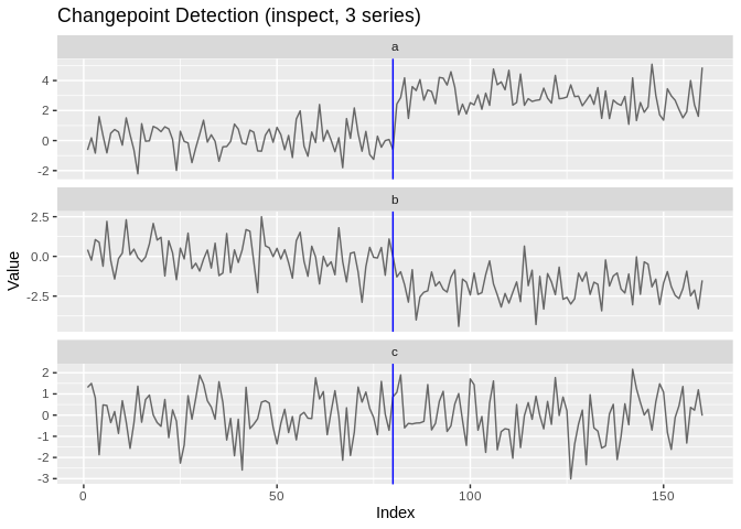
Univariate methods never silently flatten a matrix: hand one to
pelt and you get an error naming the multivariate
alternatives instead. ocd_wrapper() insists the other way:
it projects across coordinates, so it needs a matrix with at least two
columns.
When ground truth changepoints are known, compute accuracy metrics
(precision/recall/F1 under one-to-one matching within a tolerance
margin, the covering metric, Hausdorff distance, adjusted
Rand index):
# 98 matches the true changepoint at 100; 150 is a false positive
cpt_metrics(pred = c(98, 150), truth = c(100), n = 200)
#> # A tibble: 1 × 12
#>       n n_pred n_truth precision recall    f1 covering hausdorff rand_index
#>   <int>  <int>   <int>     <dbl>  <dbl> <dbl>    <dbl>     <dbl>      <dbl>
#> 1   200      2       1       0.5      1 0.667     0.74        50      0.719
#> # ℹ 3 more variables: annotation_error <int>, mae_matched <dbl>,
#> #   rmse_matched <dbl>
When multiple annotation sets are available, use
cpt_metrics_annotated(), and visualise agreement with
ggcpt_eval():
cpt_metrics_annotated(c(100), list(c(100), c(101), c(99)), n = 200, margin = 5)
#> # A tibble: 1 × 7
#>       n n_annotators n_pred precision recall    f1 covering
#>   <dbl>        <int>  <int>     <dbl>  <dbl> <dbl>    <dbl>
#> 1 200 3 1 1 1 1 0.993dat <- cpt_simulate(200, changepoints = c(100), change_in = "mean",
params = c(0, 10), sd = 1)
attributes(dat)$true_changepoints
#> [1] 100rcpt() is an alias, for readers who prefer the
r* random-generation naming. Built-in test signals include
signal_blocks() (the Donoho-Johnstone blocks signal),
signal_fms(), signal_mix(),
signal_teeth() and signal_stairs(), each
carrying its known changepoints in a true_changepoints
attribute.
cpt_penalty() constructs penalty values for the methods
that take a numeric penalty. Engines differ in how they read a penalty,
and ?cpt_penalty documents each convention:
cpt_penalty("BIC", n = 200)
#> [1] 5.298317
cpt_penalty("AIC", n = 200)
#> [1] 2
cpt_penalty("Manual", value = 10)
#> [1] 10
One caveat worth knowing. pelt,
binseg, segneigh and fpop compare
the penalty against a raw segment cost when detecting a change
in mean: changepoint’s Normal cost assumes noise of
standard deviation 1, and fpop’s lambda
penalises the residual sum of squares directly. On a series with wider
noise the penalty is effectively negligible and the segmentation
shatters: on 200 observations with one true changepoint and a five-sigma
jump, pelt returns 1 changepoint at sigma = 1 but 39 at
sigma = 3 and 141 at sigma = 10 (means over 20 draws; a single draw is
not stable here). Standardise the series
(cpt_detect(scale(x)[, 1], method = "pelt")), pass a
penalty on the data’s own scale, or use
change_in = "meanvar", which estimates a variance per
segment. The other engines estimate or cancel the noise scale themselves
and are unaffected, with three exceptions: geomcp (it runs
PELT), and decafs and bocpd on very small
units. See ?cpt_detect for the full note.
For fine-grained control, each engine also has a dedicated wrapper
that exposes its own arguments and returns a ggcpt object
directly. The classic search and pruning engines:
fpop_wrapper(x, penalty = 2 * log(200))
#> ggcpt (changepoint detection result)
#>   Method:             fpop
#>   Change in:          mean
#>   Changepoints found: 1
#>   CP convention:      left
#>   Penalty:            Manual = 10.597
#>   Series length:      200
#>
#> Changepoints:
#> # A tibble: 1 × 2
#>      cp cp_value
#>   <int>    <dbl>
#> 1   100    0.467
wbs_wrapper(x, n_intervals = 2000)
#> ggcpt (changepoint detection result)
#>   Method:             wbs
#>   Change in:          mean
#>   Changepoints found: 1
#>   CP convention:      left
#>   Penalty:            sSIC
#>   Series length:      200
#>
#> Changepoints:
#> # A tibble: 1 × 2
#>      cp cp_value
#>   <int>    <dbl>
#> 1   100    0.467
wbs2_wrapper(x)
#> ggcpt (changepoint detection result)
#>   Method:             wbs2
#>   Change in:          mean
#>   Changepoints found: 1
#>   CP convention:      left
#>   Penalty:            SDLL
#>   Series length:      200
#>
#> Changepoints:
#> # A tibble: 1 × 2
#>      cp cp_value
#>   <int>    <dbl>
#> 1   100    0.467
not_wrapper(x, contrast = "pcwsConstMean")
#> ggcpt (changepoint detection result)
#>   Method:             not
#>   Change in:          mean
#>   Changepoints found: 1
#>   CP convention:      left
#>   Penalty:            sSIC
#>   Series length:      200
#>
#> Changepoints:
#> # A tibble: 1 × 2
#>      cp cp_value
#>   <int>    <dbl>
#> 1   100    0.467
mosum_wrapper(x)
#> ggcpt (changepoint detection result)
#>   Method:             mosum
#>   Change in:          mean
#>   Changepoints found: 1
#>   CP convention:      left
#>   Penalty:            threshold = 3.6342
#>   Series length:      200
#>
#> Changepoints:
#> # A tibble: 1 × 2
#>      cp cp_value
#>   <int>    <dbl>
#> 1   100    0.467
idetect_wrapper(x)
#> ggcpt (changepoint detection result)
#>   Method:             idetect
#>   Change in:          mean
#>   Changepoints found: 1
#>   CP convention:      left
#>   Penalty:            threshold
#>   Series length:      200
#>
#> Changepoints:
#> # A tibble: 1 × 2
#>      cp cp_value
#>   <int>    <dbl>
#> 1   100    0.467
tguh_wrapper(x)
#> ggcpt (changepoint detection result)
#>   Method:             tguh
#>   Change in:          mean
#>   Changepoints found: 1
#>   CP convention:      left
#>   Penalty:            sSIC
#>   Series length:      200
#>
#> Changepoints:
#> # A tibble: 1 × 2
#>      cp cp_value
#>   <int>    <dbl>
#> 1   100    0.467
And the 0.4.0 wave (each behind its Suggests engine):
smuce_wrapper(), cpop_wrapper(),
bcp_wrapper(), bocpd_wrapper(),
beast_wrapper(), cpm_wrapper(),
kcp_wrapper(), npmojo_wrapper(),
decafs_wrapper(), sn_wrapper(),
inspect_wrapper(), ocd_wrapper(),
geomcp_wrapper(), strucchange_wrapper(),
segmented_wrapper(), envcpt_wrapper(), and
fastcpd_wrapper().
The 0.5.0 wave adds nsp_wrapper(),
mcp_wrapper(), esac_wrapper(),
pilliat_wrapper(), hdcov_wrapper(),
network_wrapper(), var_wrapper(),
fmean_wrapper(), fcov_wrapper(),
kwc_wrapper(), fabisearch_wrapper(),
wbsts_wrapper(), bfast_wrapper(),
trend_wrapper(), taylor_wrapper(),
hdreg_wrapper() and binsegrcpp_wrapper().
set.seed(2027)  # local, so this example does not depend on the chunks above
# change-in-slope: exact penalised broken-line estimation
y_slope <- cumsum(c(rep(0.4, 100), rep(-0.3, 100))) + rnorm(200)
res_slope <- cpop_wrapper(y_slope)
autoplot(res_slope, show_fit = TRUE)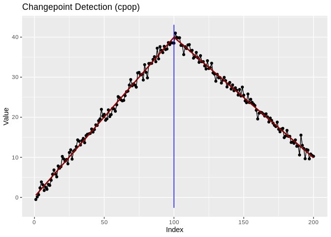
The package provides composable ggplot2 layers for changepoint visualisation:
library(ggplot2)

# Use geom_changepoint as a standalone layer
cp_tbl <- tidy(cpt_detect(x, method = "pelt", change_in = "mean"))
ggplot(data.frame(index = seq_along(x), value = x), aes(index, value)) +
  geom_line() +
  geom_changepoint(data = cp_tbl, aes(xintercept = cp), color = "red") +
  theme_ggcpt()

# Use stat_changepoint to compute and draw changepoints in one step
ggplot(data.frame(index = seq_along(x), value = x), aes(index, value)) +
  geom_line() +
  stat_changepoint(method = "pelt", color = "red")

# Shade alternating segments between changepoints
ggplot(data.frame(index = seq_along(x), value = x), aes(index, value)) +
  geom_line() +
  annotate_segments(cp = cp_tbl$cp, n = length(x))

# Draw each segment's estimated level with geom_cpt_segment
segs <- cpt_detect(x, method = "pelt", change_in = "mean")$segments
ggplot(data.frame(index = seq_along(x), value = x), aes(index, value)) +
  geom_line() +
  geom_cpt_segment(data = segs,
                   aes(x = start, xend = end,
                       y = param_estimate, yend = param_estimate),
                   color = "blue", linewidth = 1)

# Draw confidence intervals with geom_cpt_ci (when the engine provides them)
cp_ci <- tidy(smuce_wrapper(x))
ggplot(data.frame(index = seq_along(x), value = x), aes(index, value)) +
  geom_line() +
  geom_cpt_ci(data = cp_ci,
              aes(x = cp, xmin = ci_lower, xmax = ci_upper, y = min(x) - 1))

# Shade an interval that provably contains a change with geom_cpt_region,
# and mark known external events with geom_cpt_event
ggplot(data.frame(index = seq_along(x), value = x), aes(index, value)) +
  geom_cpt_region(aes(xmin = start, xmax = end),
                  data = cpt_regions(cpt_detect(x, method = "nsp"))) +
  geom_line() +
  geom_cpt_event(aes(xintercept = when, label = what),
                 data = data.frame(when = 100, what = "policy change"))
Colour is never the only channel carrying meaning.
scale_colour_cpt() (and its scale_color_cpt()
alias), scale_fill_cpt() and
scale_linetype_cpt() are the Okabe-Ito palette used
throughout, safe under deuteranopia, protanopia and tritanopia;
scale_colour_cpt_label() is the matching discrete scale for
the label-error vocabulary. Every autoplot() also carries
generated alt text, so a rendered figure reaches a screen reader without
the author writing anything.
Any result (or any ggplot built from one) renders as an interactive
widget with ggcpt_interactive() (requires
plotly). cpt_cite() returns the methodological
reference behind a result, so an analysis can cite the right paper
without leaving R:
cpt_cite("pelt")
#> [pelt] Killick, R., Fearnhead, P. and Eckley, I. A. (2012). Optimal detection of changepoints with a linear computational cost. Journal of the American Statistical Association, 107(500), 1590-1598.ggcpt_interactive(res) # hover for values; requires plotlyAdvanced users can construct ggcpt objects directly or
test for the class:
set.seed(2028)  # local, so this example does not depend on the chunks above
new_ggcpt(
  changepoints = tibble::tibble(cp = 100L, cp_value = 5.0),
  data = tibble::tibble(index = 1:200, value = rnorm(200)),
  method = "manual"
)
is_ggcpt(res)cpt_wrapper(), ecp_wrapper(),
ggcptplot() and ggecpplot() all continue to
work unchanged. ecp_wrapper() and ggecpplot()
reach the ecp engine directly, including genuine
multivariate input:
ecp_wrapper(x, algorithm = "divisive")
ggecpplot(x, algorithm = "divisive")cpt_wrapper(x)
#> # A tibble: 1 × 2
#> cp cp_value
#> <int> <dbl>
#> 1 100 0.467
ggcptplot(x)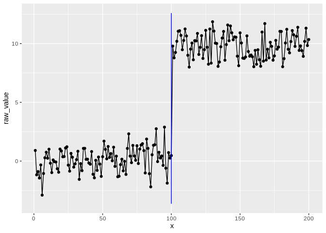
The ggcpt class also provides:
res <- cpt_detect(x, method = "pelt", change_in = "mean")
summary(res)          # human-readable digest
#> ggcpt Summary
#>   Method:             pelt
#>   Change in:          mean
#>   Changepoints found: 1
#>   CP convention:      left
#>   Series length:      200
#>   Penalty:            MBIC
#>   Runtime (seconds):  0.019
#>
#> Segments:
#> # A tibble: 2 × 5
#>   seg_id start   end     n param_estimate
#>    <int> <int> <int> <int>          <dbl>
#> 1      1     1   100   100          0.139
#> 2      2   101   200   100          9.80
#>
#> Changepoints:
#> # A tibble: 1 × 2
#>      cp cp_value
#>   <int>    <dbl>
#> 1   100    0.467
as_tibble(res)        # tibble of changepoints
#> # A tibble: 1 × 2
#>      cp cp_value
#>   <int>    <dbl>
#> 1   100    0.467
as.data.frame(res)    # data frame of changepoints
#>    cp cp_value
#> 1 100 0.467023
format(res)           # one-line summary string
#> [1] "ggcpt [pelt] 1 changepoint(s) on 200 observations"
plot(res)             # base-graphics fallback (delegates to autoplot)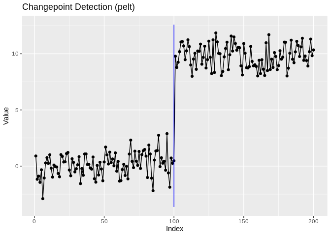
The full reference index and rendered vignettes live at https://pursuitofdatascience.github.io/ggchangepoint/. From R:
vignette("ggchangepoint", package = "ggchangepoint"):
feature tourvignette("introduction", package = "ggchangepoint"):
the framework, in research-paper formvignette("comparison", package = "ggchangepoint"):
method comparison and evaluation