
Web: https://jangelini.github.io/geneticae/
CRAN: https://CRAN.R-project.org/package=geneticae/index.html
![]()
Understanding the relationship between crops performance and environment is a key problem for plant breeders and geneticists. In advanced stages of breeding programs, in which few genotypes are evaluated, multi-environmental trials (MET) are one of the most used experiments. Such studies test a number of genotypes in multiple environments in order to identify the superior genotypes according to their performance. In these experimentes, crop performance is modeled as a function of genotype (G), environment (E) and genotype-environment interaction (GEI). The presence of GEI generates differential genotypic responses in the different environments. Therefore appropriate statistical methods should be used to obtain an adequate GEI analysis, which is essential for plant breeders.
The average performance of genotypes through different environments can only be considered in the absence of GEI. However, GEI is almost always present and the comparison of the mean performance between genotypes is not enough. The most widely used methods to analyze MET data are based on regression models, analysis of variance (ANOVA) and multivariate techniques. In particular, two statistical models are widely used among plant breeders as they provide useful graphical tools for the study of GEI: the Additive Main effects and Multiplicative Interaction model (AMMI) and the Site Regression Model (SREG). However, these models are not always efficient enough to analyze MET data structure of plant breeding programs. They present serious limitations in the presence of atypical observations and missing values, which occur very frequently. To overcome this, several imputation alternatives (Angelini et al., 2024) and a robust AMMI and a SREG model were recently proposed in literature (Rodrigues et al., 2016; Angelini et al., 2022).
The geneticae package was created to gather in one place
the most useful functions for this type of analysis and it also
implements new methodology which can be found in recent literature. More
importantly, geneticae is the first package to implement
the robust AMMI models proposed by Rodrigues et al. (2016), the robusts
SREG proposed by Angelini et al. (2022) and new imputation methods
proposed by Angelini et al. (2024). In addition, there is no need to
preprocess the data to use the geneticae package, as it the
case of some previous packages which require a data frame or matrix
containing genotype by environment means with the genotypes in rows and
the environments in columns. In this package, data in long format is
required. There is no restriction on columns names of genotypes,
environments, repetitions (if any) and phenotypic traits of interest.
Also, extra information that will not be used in the analysis may be
present in the dataset. Finally, geneticae offers a wide
variety of options to customize the biplots, which are part of the
graphical output of these methods.
This package can be used through this Shiny app, making it available not only for R programmers.
You can install the released version of geneticae from
CRAN with:
install.packages("geneticae")You can install the development version from our GitHub repo with:
# install.packages("devtools")
devtools::install_github("jangelini/geneticae")You can use geneticae through this
Shiny app. Source code is in GitHub
repo.
If you are just getting started with geneticae we
recommend visiting the vignettes and exploring the examples throughout
the package documentation.
Here we present a small example.
The dataset yan.winterwheat has information about the
yield of 18 winter wheat varieties grown in nine environments in Ontario
at 1993. The function GGEPlot() builds several GGE biplots
views. The basic biplot is produced with the argument
type="Biplot". If the function is used with the argument
type = "Selected Environment" and the name of one
environment is provided in selectedE, a line that passes
through the environment marker (i.e. OA93), and the biplot origin is
added. The most suitable cultivars for that particular environment can
be identified looking at their projection onto this axis. Thus, at the
environment OA93, the highest-yielding cultivar was Zav, and
the lowest-yielding cultivar was Luc. The perpendicular line to
the OA93 axis separates genotypes that yielded above and below the mean
in this environment.
library(geneticae)
library(agridat)
data(yan.winterwheat)


GGE1 <- rSREGModel(yan.winterwheat, genotype = "gen", environment = "env",
                   response = "yield",  model = "SREG")

rSREGPlot(GGE1, type = "Selected Environment", selectedE = "OA93", footnote = FALSE, titles = FALSE)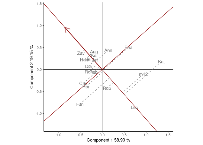
Figure: comparison of cultivar performance in a selected environment.