A package for estimation, forecasting, and simulation of generalized autoregressive score (GAS) models of Creal et al. (2013) and Harvey (2013), also known as dynamic conditional score (DCS) models or score-driven (SD) models.
Model specification allows for various conditional distributions, different parametrizations, exogenous variables, higher score and autoregressive orders, custom and unconditional initial values of time-varying parameters, fixed and bounded values of coefficients, and missing values. Model estimation is performed by the maximum likelihood method.
The package offers the following functions for working with GAS models:
gas() estimates GAS models.gas_simulate() simulates GAS models.gas_forecast() forecasts GAS models.gas_filter() obtains filtered time-varying parameters
of GAS models.gas_bootstrap() bootstraps coefficients of GAS
models.The package handles probability distributions by the following functions:
distr() provides table of supported distributions.distr_density() computes the density of a given
distribution.distr_mean() computes the mean of a given
distribution.distr_var() computes the variance of a given
distribution.distr_score() computes the score of a given
distribution.distr_fisher() computes the Fisher information of a
given distribution.distr_random() generates random observations from a
given distribution.In addition, the package provides the following datasets used in examples:
bookshop_orders contains times of antiquarian bookshop
orders.ice_hockey_championships contains the results of the
Ice Hockey World Championships.toilet_paper_sales contains daily sales of toilet
paper.To install the gasmodel package from CRAN, you can
use:
install.packages("gasmodel")To install the development version of the gasmodel
package from GitHub, you can use:
install.packages("devtools")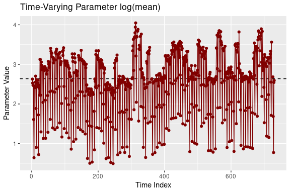
devtools::install_github("vladimirholy/gasmodel")As a simple example, let us model daily toilet paper sales in a store. We estimate the GAS model based on the negative binomial distribution with time-varying mean and incorporating dummy variables to indicate the day of the week and whether the product is being promoted. We also plot the filtered time-varying parameters:
library("gasmodel")

data("toilet_paper_sales")
y <- toilet_paper_sales$quantity
x <- as.matrix(toilet_paper_sales[3:9])

est_negbin <- gas(y = y, x = x, distr = "negbin", regress = "sep")
est_negbin
#> GAS Model: Negative Binomial Distribution / NB2 Parametrization / Unit Scaling
#>
#> Coefficients:
#>                    Estimate Std. Error   Z-Test  Pr(>|Z|)
#> log(mean)_omega   2.6384526  0.0562032  46.9449 < 2.2e-16 ***
#> log(mean)_beta1  -0.0100824  0.0357634  -0.2819   0.77800
#> log(mean)_beta2  -0.0772088  0.0366240  -2.1081   0.03502 *
#> log(mean)_beta3  -0.0155342  0.0361813  -0.4293   0.66767
#> log(mean)_beta4   0.0452482  0.0357004   1.2674   0.20500
#> log(mean)_beta5  -0.8240699  0.0430441 -19.1448 < 2.2e-16 ***
#> log(mean)_beta6  -1.7736613  0.0589493 -30.0879 < 2.2e-16 ***
#> log(mean)_beta7   0.7037864  0.0481655  14.6118 < 2.2e-16 ***
#> log(mean)_alpha1  0.0256734  0.0035329   7.2670 3.676e-13 ***
#> log(mean)_phi1    0.9769718  0.0175857  55.5549 < 2.2e-16 ***
#> dispersion        0.0349699  0.0051488   6.7918 1.107e-11 ***
#> ---
#> Signif. codes:  0 '***' 0.001 '**' 0.01 '*' 0.05 '.' 0.1 ' ' 1
#>
#> Log-Likelihood: -2059.834, AIC: 4141.668, BIC: 4191.824

plot(est_negbin)
To further illustrate the usability of GAS models, the package includes the following case studies in the form of vignettes:
case_durations analyzes the timing of online
antiquarian bookshop orders.case_rankings analyzes the strength of national ice
hockey teams using the annual Ice Hockey World Championships
rankings.Currently, there are 36 distributions available.
The list of supported distribution can be obtained by the
distr() function:
| Label | Distribution | Dimension | Data Type | Parametrizations |
|---|---|---|---|---|
| alaplace | Asymmetric Laplace | Univariate | Real | meanscale |
| bernoulli | Bernoulli | Univariate | Binary | prob |
| beta | Beta | Univariate | Interval | conc, meansize, meanvar |
| bisa | Birnbaum-Saunders | Univariate | Duration | scale |
| burr | Burr | Univariate | Duration | scale |
| cat | Categorical | Multivariate | Categorical | worth |
| dirichlet | Dirichlet | Multivariate | Compositional | conc |
| dpois | Double Poisson | Univariate | Count | mean |
| exp | Exponential | Univariate | Duration | scale, rate |
| explog | Exponential-Logarithmic | Univariate | Duration | rate |
| fisk | Fisk | Univariate | Duration | scale |
| gamma | Gamma | Univariate | Duration | scale, rate |
| ged | Generalized Error | Univariate | Real | meanscale |
| gengamma | Generalized Gamma | Univariate | Duration | scale, rate |
| geom | Geometric | Univariate | Count | mean, prob |
| kuma | Kumaraswamy | Univariate | Interval | conc |
| laplace | Laplace | Univariate | Real | meanscale |
| logistic | Logistic | Univariate | Real | meanscale |
| logitnorm | Logit-Normal | Univariate | Interval | logitmeanvar |
| lognorm | Log-Normal | Univariate | Duration | logmeanvar |
| lomax | Lomax | Univariate | Duration | scale |
| mvnorm | Multivariate Normal | Multivariate | Real | meanvar |
| mvt | Multivariate Student’s t | Multivariate | Real | meanvar |
| negbin | Negative Binomial | Univariate | Count | nb2, prob |
| norm | Normal | Univariate | Real | meanvar |
| pluce | Plackett-Luce | Multivariate | Ranking | worth |
| pois | Poisson | Univariate | Count | mean |
| rayleigh | Rayleigh | Univariate | Duration | scale |
| skellam | Skellam | Univariate | Integer | meanvar, diff, meandisp |
| t | Student’s t | Univariate | Real | meanvar |
| vonmises | von Mises | Univariate | Circular | meanconc |
| weibull | Weibull | Univariate | Duration | scale, rate |
| zigeom | Zero-Inflated Geometric | Univariate | Count | mean |
| zinegbin | Zero-Inflated Negative Binomial | Univariate | Count | nb2 |
| zipois | Zero-Inflated Poisson | Univariate | Count | mean |
| ziskellam | Zero-Inflated Skellam | Univariate | Integer | meanvar, diff, meandisp |
Details of each distribution, including its density function,
expected value, variance, score, and Fisher information, can be found in
vignette distributions.
The generalized autoregressive score (GAS) models of Creal et al. (2013) and Harvey (2013), also known as dynamic conditional score (DCS) models or score-driven (SD) models, have established themselves as a useful modern framework for time series modeling.
The GAS models are observation-driven models allowing for any underlying probability distribution \(p(y_t|f_t)\) with any time-varying parameters \(f_t\) for time series \(y_t\). They capture the dynamics of time-varying parameters using the autoregressive term and the lagged score, i.e. the gradient of the log-likelihood function. Exogenous variables can also be included. Specifically, time-varying parameters \(f_{t}\) follow the recursion \[f_{t} = \omega + \sum_{i=1}^M \beta_i x_{ti} + \sum_{j=1}^P \alpha_j S(f_{t - j}) \nabla(y_{t - j}, f_{t - j}) + \sum_{k=1}^Q \varphi_k f_{t-k},\] where \(\omega\) is the intercept, \(\beta_i\) are the regression parameters, \(\alpha_j\) are the score parameters, \(\varphi_k\) are the autoregressive parameters, \(x_{ti}\) are the exogenous variables, \(S(f_t)\) is a scaling function for the score, and \(\nabla(y_t, f_t)\) is the score given by \[\nabla(y_t, f_t) = \frac{\partial \ln p(y_t | f_t)}{\partial f_t}.\] In the case of a single time-varying parameter, \(\omega\), \(\beta_i\), \(\alpha_j\), \(\varphi_k\), \(x_{ti}\), \(S(f_t)\), and \(\nabla(y_t, f_t)\) are all scalar. In the case of multiple time-varying parameters, \(x_{ti}\) are scalar, \(\omega\), \(\beta_i\), and \(\nabla(y_{t - j}, f_{t - j})\) are vectors, \(\alpha_j\) and \(\varphi_k\) are diagonal matrices, and \(S(f_t)\) is a square matrix. Alternatively, a different model can be obtained by defining the recursion in the fashion of regression models with dynamic errors as \[f_{t} = \omega + \sum_{i=1}^M \beta_i x_{ti} + e_{t}, \quad e_t = \sum_{j=1}^P \alpha_j S(f_{t - j}) \nabla(y_{t - j}, f_{t - j}) + \sum_{k=1}^Q \varphi_k e_{t-k}.\]
The GAS models can be straightforwardly estimated by the maximum likelihood method. For the asymptotic theory regarding the GAS models and maximum likelihood estimation, see Blasques et al. (2014), Blasques et al. (2018), and Blasques et al. (2022).
The use of the score for updating time-varying parameters is optimal in an information theoretic sense. For an investigation of the optimality properties of GAS models, see Blasques et al. (2015) and Blasques et al. (2021).
Generally, the GAS models perform quite well when compared to alternatives, including parameter-driven models. For a comparison of the GAS models to alternative models, see Koopman et al. (2016) and Blazsek and Licht (2020).
The GAS class includes many well-known econometric models, such as the generalized autoregressive conditional heteroskedasticity (GARCH) model of Bollerslev (1986), the autoregressive conditional duration (ACD) model of Engle and Russel (1998), and the Poisson count model of Davis et al. (2003). More recently, a variety of novel score-driven models has been proposed, such as the Beta-t-(E)GARCH model of Harvey and Chakravarty (2008), a Skellam model of Koopman et al. (2018), a directional model of Harvey (2019), a bivariate Poisson model of Koopman and Lit (2019), and a ranking model of Holý and Zouhar (2022). For an overview of various GAS models, see Harvey (2022).
The extensive GAS literature is listed on www.gasmodel.com.
Blasques, F., Gorgi, P., Koopman, S. J., and Wintenberger, O. (2018). Feasible Invertibility Conditions and Maximum Likelihood Estimation for Observation-Driven Models. Electronic Journal of Statistics, 12(1), 1019–1052. doi: 10.1214/18-ejs1416.
Blasques, F., Koopman, S. J., and Lucas, A. (2014). Stationarity and Ergodicity of Univariate Generalized Autoregressive Score Processes. Electronic Journal of Statistics, 8(1), 1088–1112. doi: 10.1214/14-ejs924.
Blasques, F., Koopman, S. J., and Lucas, A. (2015). Information-Theoretic Optimality of Observation-Driven Time Series Models for Continuous Responses. Biometrika, 102(2), 325–343. doi: 10.1093/biomet/asu076.
Blasques, F., Lucas, A., and van Vlodrop, A. C. (2021). Finite Sample Optimality of Score-Driven Volatility Models: Some Monte Carlo Evidence. Econometrics and Statistics, 19, 47–57. doi: 10.1016/j.ecosta.2020.03.010.
Blasques, F., van Brummelen, J., Koopman, S. J., and Lucas, A. (2022). Maximum Likelihood Estimation for Score-Driven Models. Journal of Econometrics, 227(2), 325–346. doi: 10.1016/j.jeconom.2021.06.003.
Blazsek, S. and Licht, A. (2020). Dynamic Conditional Score Models: A Review of Their Applications. Applied Economics, 52(11), 1181–1199. doi: 10.1080/00036846.2019.1659498.
Bollerslev, T. (1986). Generalized Autoregressive Conditional Heteroskedasticity. Journal of Econometrics, 31(3), 307–327. doi: 10.1016/0304-4076(86)90063-1.
Creal, D., Koopman, S. J., and Lucas, A. (2013). Generalized Autoregressive Score Models with Applications. Journal of Applied Econometrics, 28(5), 777–795. doi: 10.1002/jae.1279.
Davis, R. A., Dunsmuir, W. T. M., and Street, S. B. (2003). Observation-Driven Models for Poisson Counts. Biometrika, 90(4), 777–790. doi: 10.1093/biomet/90.4.777.
Engle, R. F. and Russell, J. R. (1998). Autoregressive Conditional Duration: A New Model for Irregularly Spaced Transaction Data. Econometrica, 66(5), 1127–1162. doi: 10.2307/2999632.
Harvey, A. C. (2013). Dynamic Models for Volatility and Heavy Tails: With Applications to Financial and Economic Time Series. Cambridge University Press. doi: 10.1017/cbo9781139540933.
Harvey, A. C. (2022). Score-Driven Time Series Models. Annual Review of Statistics and Its Application, 9(1), 321–342. doi: 10.1146/annurev-statistics-040120-021023.
Harvey, A. C. and Chakravarty, T. (2008). Beta-t-(E)GARCH. Cambridge Working Papers in Economics, CWPE 0840. doi: 10.17863/cam.5286.
Harvey, A., Hurn, S., and Thiele, S. (2019). Modeling Directional (Circular) Time Series. Cambridge Working Papers in Economics, CWPE 1971. doi: 10.17863/cam.43915.
Holý, V. and Zouhar, J. (2022). Modelling Time-Varying Rankings with Autoregressive and Score-Driven Dynamics. Journal of the Royal Statistical Society: Series C (Applied Statistics), 71(5). doi: 10.1111/rssc.12584.
Koopman, S. J. and Lit, R. (2019). Forecasting Football Match Results in National League Competitions Using Score-Driven Time Series Models. International Journal of Forecasting, 35(2), 797–809. doi: 10.1016/j.ijforecast.2018.10.011.
Koopman, S. J., Lit, R., Lucas, A., and Opschoor, A. (2018). Dynamic Discrete Copula Models for High-Frequency Stock Price Changes. Journal of Applied Econometrics, 33(7), 966–985. doi: 10.1002/jae.2645.
Koopman, S. J., Lucas, A., and Scharth, M. (2016). Predicting Time-Varying Parameters with Parameter-Driven and Observation-Driven Models. Review of Economics and Statistics, 98(1), 97–110. doi: 10.1162/rest_a_00533.