![]()
![]()
![]()
![]()
Fast Robust Moments – Pick Three!
Fast, numerically robust, higher order moments in R, computed via Rcpp, mostly as an exercise to learn Rcpp. Supports computation on vectors and matrices, and Monoidal append (and unappend) of moments. Computations are via the Welford-Terriberry algorithm, as described by Bennett et al.
– Steven E. Pav, shabbychef@gmail.com
This package can be installed from CRAN, via drat, or from github:
# via CRAN:
install.packages("fromo")
# via drat:
if (require(drat)) {
    drat:::add("shabbychef")
    install.packages("fromo")
}
# get snapshot from github (may be buggy)
if (require(devtools)) {
    install_github("shabbychef/fromo")
}Currently the package functionality can be divided into the following: * Functions which reduce a vector to an array of moments. * Functions which take a vector to a matrix of the running moments. * Functions which transform a vector to some normalized form, like a centered, rescaled, z-scored sample, or a summarized form, like the running Sharpe or t-stat. * Functions for computing the covariance of a vector robustly. * Object representations of moments with join and unjoin methods.
A function which computes, say, the kurtosis, typically also computes the mean and standard deviation, and has performed enough computation to easily return the skew. However, the default functions in R for higher order moments discard these lower order moments. So, for example, if you wish to compute Merten’s form for the standard error of the Sharpe ratio, you have to call separate functions to compute the kurtosis, skew, standard deviation, and mean.
The summary functions in fromo return all the
moments up to some order, namely the functions sd3,
skew4, and kurt5. The latter of these,
kurt5 returns an array of length 5 containing the
excess kurtosis, the skewness, the standard deviation, the
mean, and the observation count. (The number in the function name
denotes the length of the output.) Along the same lines, there are
summarizing functions that compute centered moments, standardized
moments, and ‘raw’ cumulants:
cent_moments: return a k+1-vector of the
kth centered moment, the k-1th, all the way
down to the 2nd (the variance), then the mean and the
observation count.std_moments: return a k+1-vector of the
kth standardized moment, the k-1th, all the
way down to the 3rd, then the standard deviation, the mean, and
the observation count.cent_cumulants: computes the centered cumulants (yes,
this is redundant, but they are not standardized). return a
k+1-vector of the kth raw cumulant, the
k-1th, all the way down to the second, then the mean, and
the observation count.std_cumulants: computes the standardized (and, of
course, centered) cumulants. return a k+1-vector of the
kth standardized cumulant, all the way down to the third,
then the variance, the mean, and the observation count.library(fromo)
set.seed(12345)
x <- rnorm(1000, mean = 10, sd = 2)
show(cent_moments(x, max_order = 4, na_rm = TRUE))## [1] 47.276 -0.047 3.986 10.092 1000.000show(std_moments(x, max_order = 4, na_rm = TRUE))## [1] 3.0e+00 -5.9e-03 2.0e+00 1.0e+01 1.0e+03show(cent_cumulants(x, max_order = 4, na_rm = TRUE))## [1] -0.388 -0.047 3.986 10.092 1000.000show(std_cumulants(x, max_order = 4, na_rm = TRUE))## [1] -2.4e-02 -5.9e-03 4.0e+00 1.0e+01 1.0e+03In theory these operations should be just as fast as the default functions, but faster than calling multiple default functions. Here is a speed comparison of the basic moment computations:
library(fromo)
library(moments)
library(microbenchmark)

set.seed(1234)
x <- rnorm(1000)

dumbk <- function(x) {
    c(kurtosis(x) - 3, skewness(x), sd(x), mean(x),
        length(x))
}

microbenchmark(kurt5(x), skew4(x), sd3(x), dumbk(x),
    kurtosis(x), skewness(x), sd(x), mean(x))
## Unit: microseconds
## expr min lq mean median uq max neval cld
## kurt5(x) 80.5 81.4 87.0 82 84.1 162 100 a
## skew4(x) 69.2 70.0 73.9 71 71.9 117 100 a
## sd3(x) 12.4 13.1 13.8 13 13.8 35 100 b
## dumbk(x) 98.1 99.6 142.2 101 108.4 3322 100 c
## kurtosis(x) 40.3 41.3 46.1 42 43.5 215 100 ab
## skewness(x) 39.6 41.1 42.8 42 42.7 72 100 ab
## sd(x) 9.6 10.5 11.4 11 11.4 24 100 b
## mean(x) 4.2 4.7 5.1 5 5.3 15 100 bx <- rnorm(1e+07, mean = 1e+12)
microbenchmark(kurt5(x), skew4(x), sd3(x), dumbk(x),
kurtosis(x), skewness(x), sd(x), mean(x), times = 10L)## Unit: milliseconds
## expr min lq mean median uq max neval cld
## kurt5(x) 822 831 873 859 927 943 10 a
## skew4(x) 701 715 756 752 783 825 10 b
## sd3(x) 105 106 113 108 114 137 10 c
## dumbk(x) 893 900 982 1009 1035 1079 10 d
## kurtosis(x) 419 420 483 470 508 648 10 e
## skewness(x) 414 421 468 470 489 571 10 e
## sd(x) 38 38 42 42 44 47 10 f
## mean(x) 19 19 20 19 20 22 10 f# clean up
rm(x)Many of the methods now support the computation of weighted moments. There are a few options around weights: whether to check them for negative values, whether to normalize them to unit mean.
library(fromo)
library(moments)
library(microbenchmark)

set.seed(987)
x <- rnorm(1000)
w <- runif(length(x))

# no weights:
show(cent_moments(x, max_order = 4, na_rm = TRUE))
## [1] 2.9e+00 1.2e-02 1.0e+00 1.0e-02 1.0e+03# with weights:
show(cent_moments(x, max_order = 4, wts = w, na_rm = TRUE))## [1] 3.1e+00 4.1e-02 1.0e+00 1.3e-02 1.0e+03# if you turn off weight normalization, the last
# element is sum(wts):
show(cent_moments(x, max_order = 4, wts = w, na_rm = TRUE,
normalize_wts = FALSE))## [1] 3.072 0.041 1.001 0.013 493.941# let's compare for speed!
x <- rnorm(1e+07)
w <- runif(length(x))
slow_sd <- function(x, w) {
n0 <- length(x)
mu <- weighted.mean(x, w = w)
sg <- sqrt(sum(w * (x - mu)^2)/(n0 - 1))
c(sg, mu, n0)
}
microbenchmark(sd3(x, wts = w), slow_sd(x, w))## Unit: milliseconds
## expr min lq mean median uq max neval cld
## sd3(x, wts = w) 120 125 133 130 136 180 100 a
## slow_sd(x, w) 235 277 318 294 329 575 100 b# clean up
rm(x, w)The as.centsums object performs the summary
(centralized) moment computation, and stores the centralized sums. There
is a print method that shows raw, centralized, and standardized moments
of the ingested data. This object supports concatenation and
unconcatenation. These should satisfy ‘monoidal homomorphism’, meaning
that concatenation and taking moments commute with each other. So if you
have two vectors, x1 and x2, the following
should be equal: c(as.centsums(x1,4),as.centsums(x2,4)) and
as.centsums(c(x1,x2),4). Moreover, the following should
also be equal:
as.centsums(c(x1,x2),4) %-% as.centsums(x2,4)) and
as.centsums(x1,4). This is a small step of the way towards
fast machine learning methods (along the lines of Mike Izbicki’s Hlearn library).
Some demo code:
set.seed(12345)
x1 <- runif(100)
x2 <- rnorm(100, mean = 1)
max_ord <- 6L

obj1 <- as.centsums(x1, max_ord)
# display:
show(obj1)
## class: centsums
## raw moments: 100 0.0051 0.09 -0.00092 0.014 -0.00043 0.0027
## central moments: 0 0.09 -0.0023 0.014 -0.00079 0.0027
## std moments: 0 1 -0.086 1.8 -0.33 3.8# join them together
obj1 <- as.centsums(x1, max_ord)
obj2 <- as.centsums(x2, max_ord)
obj3 <- as.centsums(c(x1, x2), max_ord)
alt3 <- c(obj1, obj2)
# it commutes!
stopifnot(max(abs(sums(obj3) - sums(alt3))) < 1e-07)
# unjoin them, with this one weird operator:
alt2 <- obj3 %-% obj1
alt1 <- obj3 %-% obj2
stopifnot(max(abs(sums(obj2) - sums(alt2))) < 1e-07)
stopifnot(max(abs(sums(obj1) - sums(alt1))) < 1e-07)We also have ‘raw’ join and unjoin methods, not nicely wrapped:
set.seed(123)
x1 <- rnorm(1000, mean = 1)
x2 <- rnorm(1000, mean = 1)
max_ord <- 6L
rs1 <- cent_sums(x1, max_ord)
rs2 <- cent_sums(x2, max_ord)
rs3 <- cent_sums(c(x1, x2), max_ord)
rs3alt <- join_cent_sums(rs1, rs2)
stopifnot(max(abs(rs3 - rs3alt)) < 1e-07)

rs1alt <- unjoin_cent_sums(rs3, rs2)
rs2alt <- unjoin_cent_sums(rs3, rs1)
stopifnot(max(abs(rs1 - rs1alt)) < 1e-07)
stopifnot(max(abs(rs2 - rs2alt)) < 1e-07)There is also code for computing co-sums and co-moments, though as of this writing only up to order 2. Some demo code for the monoidal stuff here:
set.seed(54321)
x1 <- matrix(rnorm(100 * 4), ncol = 4)
x2 <- matrix(rnorm(100 * 4), ncol = 4)

max_ord <- 2L
obj1 <- as.centcosums(x1, max_ord, na.omit = TRUE)
# display:
show(obj1)
## An object of class "centcosums"
## Slot "cosums":
## [,1] [,2] [,3] [,4] [,5]
## [1,] 100.0000 -0.093 0.045 -0.0046 0.046
## [2,] -0.0934 111.012 4.941 -16.4822 6.660
## [3,] 0.0450 4.941 71.230 0.8505 5.501
## [4,] -0.0046 -16.482 0.850 117.3456 13.738
## [5,] 0.0463 6.660 5.501 13.7379 100.781
##
## Slot "order":
## [1] 2# join them together
obj1 <- as.centcosums(x1, max_ord)
obj2 <- as.centcosums(x2, max_ord)
obj3 <- as.centcosums(rbind(x1, x2), max_ord)
alt3 <- c(obj1, obj2)
# it commutes!
stopifnot(max(abs(cosums(obj3) - cosums(alt3))) < 1e-07)
# unjoin them, with this one weird operator:
alt2 <- obj3 %-% obj1
alt1 <- obj3 %-% obj2
stopifnot(max(abs(cosums(obj2) - cosums(alt2))) < 1e-07)
stopifnot(max(abs(cosums(obj1) - cosums(alt1))) < 1e-07)Since an online algorithm is used, we can compute cumulative running moments. Moreover, we can remove observations, and thus compute moments over a fixed length lookback window. The code checks for negative even moments caused by roundoff, and restarts the computation to correct; periodic recomputation can be forced by an input parameter.
A demonstration:
library(fromo)
library(moments)
library(microbenchmark)

set.seed(1234)
x <- rnorm(20)

k5 <- running_kurt5(x, window = 10L)
colnames(k5) <- c("excess_kurtosis", "skew", "stdev",
    "mean", "nobs")
k5
## excess_kurtosis skew stdev mean nobs
## [1,] NaN NaN NaN -1.207 1
## [2,] NaN NaN 1.05 -0.465 2
## [3,] NaN -0.34 1.16 0.052 3
## [4,] -1.520 -0.13 1.53 -0.548 4
## [5,] -1.254 -0.50 1.39 -0.352 5
## [6,] -0.860 -0.79 1.30 -0.209 6
## [7,] -0.714 -0.70 1.19 -0.261 7
## [8,] -0.525 -0.64 1.11 -0.297 8
## [9,] -0.331 -0.58 1.04 -0.327 9
## [10,] -0.331 -0.42 1.00 -0.383 10
## [11,] 0.262 -0.65 0.95 -0.310 10
## [12,] 0.017 -0.30 0.95 -0.438 10
## [13,] 0.699 -0.61 0.79 -0.624 10
## [14,] -0.939 0.69 0.53 -0.383 10
## [15,] -0.296 0.99 0.64 -0.330 10
## [16,] 1.078 1.33 0.57 -0.391 10
## [17,] 1.069 1.32 0.57 -0.385 10
## [18,] 0.868 1.29 0.60 -0.421 10
## [19,] 0.799 1.31 0.61 -0.449 10
## [20,] 1.193 1.50 1.07 -0.118 10# trust but verify
alt5 <- sapply(seq_along(x), function(iii) {
rowi <- max(1, iii - 10 + 1)
kurtosis(x[rowi:iii]) - 3
}, simplify = TRUE)
cbind(alt5, k5[, 1])## alt5
## [1,] NaN NaN
## [2,] -2.000 NaN
## [3,] -1.500 NaN
## [4,] -1.520 -1.520
## [5,] -1.254 -1.254
## [6,] -0.860 -0.860
## [7,] -0.714 -0.714
## [8,] -0.525 -0.525
## [9,] -0.331 -0.331
## [10,] -0.331 -0.331
## [11,] 0.262 0.262
## [12,] 0.017 0.017
## [13,] 0.699 0.699
## [14,] -0.939 -0.939
## [15,] -0.296 -0.296
## [16,] 1.078 1.078
## [17,] 1.069 1.069
## [18,] 0.868 0.868
## [19,] 0.799 0.799
## [20,] 1.193 1.193If you like rolling computations, do also check out the following packages (I believe they are all on CRAN):
Of these three, it seems that RollingWindow implements
the optimal algorithm of reusing computations, while the other two
packages gain efficiency from parallelization and implementation in
C++.
Through template magic, the same code was modified to perform running centering, scaling, z-scoring and so on:
library(fromo)
library(moments)
library(microbenchmark)

set.seed(1234)
x <- rnorm(20)

xz <- running_zscored(x, window = 10L)

# trust but verify
altz <- sapply(seq_along(x), function(iii) {
    rowi <- max(1, iii - 10 + 1)
    (x[iii] - mean(x[rowi:iii]))/sd(x[rowi:iii])
}, simplify = TRUE)

cbind(xz, altz)
## altz
## [1,] NaN NA
## [2,] 0.71 0.71
## [3,] 0.89 0.89
## [4,] -1.18 -1.18
## [5,] 0.56 0.56
## [6,] 0.55 0.55
## [7,] -0.26 -0.26
## [8,] -0.23 -0.23
## [9,] -0.23 -0.23
## [10,] -0.51 -0.51
## [11,] -0.17 -0.17
## [12,] -0.59 -0.59
## [13,] -0.19 -0.19
## [14,] 0.84 0.84
## [15,] 2.02 2.02
## [16,] 0.49 0.49
## [17,] -0.22 -0.22
## [18,] -0.82 -0.82
## [19,] -0.64 -0.64
## [20,] 2.37 2.37A list of the available running functions:
running_centered : from the current value, subtract the
mean over the trailing window.running_scaled: divide the current value by the
standard deviation over the trailing window.running_zscored: from the current value, subtract the
mean then divide by the standard deviation over the trailing
window.running_sharpe: divide the mean by the standard
deviation over the trailing window. There is a boolean flag to also
compute and return the Mertens’ form of the standard error of the Sharpe
ratio over the trailing window in the second column.running_tstat: compute the t-stat over the trailing
window.running_cumulants: computes cumulants over the trailing
window.running_apx_quantiles: computes approximate quantiles
over the trailing window based on the cumulants and the Cornish-Fisher
approximation.running_apx_median: uses
running_apx_quantiles to give the approximate median over
the trailing window.The functions running_centered,
running_scaled and running_zscored take an
optional lookahead parameter that allows you to peek ahead
(or behind if negative) to the computed moments for comparing against
the current value. These are not supported for
running_sharpe or running_tstat because they
do not have an idea of the ‘current value’.
Here is an example of using the lookahead to z-score some data, compared to a purely time-safe lookback. Around a timestamp of 1000, you can see the difference in outcomes from the two methods:
set.seed(1235)
z <- rnorm(1500, mean = 0, sd = 0.09)
x <- exp(cumsum(z)) - 1

xz_look <- running_zscored(x, window = 301, lookahead = 150)
xz_safe <- running_zscored(x, window = 301, lookahead = 0)
df <- data.frame(timestamp = seq_along(x), raw = x,
    lookahead = xz_look, lookback = xz_safe)

library(tidyr)
gdf <- gather(df, key = "smoothing", value = "x", -timestamp)

library(ggplot2)
ph <- ggplot(gdf, aes(x = timestamp, y = x, group = smoothing,
    colour = smoothing)) + geom_line()
print(ph)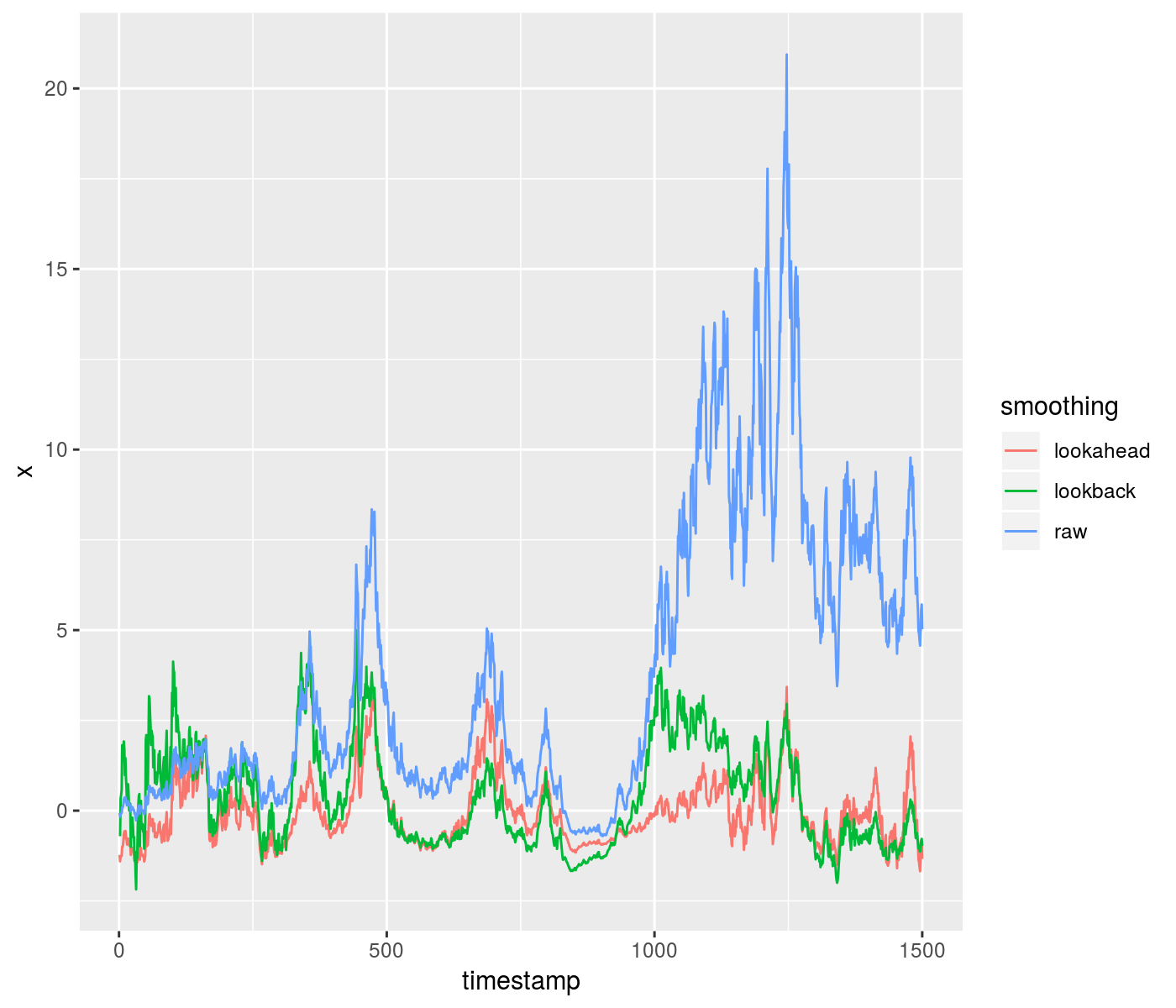
plot of chunk toy_zscore
The package now supports operations on a running window of two
aligned input series, \(x\) and \(y\), and can compute the correlation,
covariance, and OLS regression on the two over a running windo. The
following are supported: * running_correlation: the
correlation over the trailing window. * running_covariance:
the covariance of the two series. * running_covariance3:
the full variance-covariance of the two series, returning matrix with
three columns. * running_regression_intercept: the
intercept of the OLS regression fit over the trailing window. *
running_regression_slope: the slope of the OLS regression
fit over the trailing window. * running_regression_fit: a
matrix of the intercept and slope of the OLS regression fit over the
trailing window. * running_regression_diagnostics: a matrix
of the intercept and slope of the OLS regression fit, the regression
standard error and the standard errors of the intercept and slope, over
the trailing window.
The standard running moments computations listed above work on a running window of a fixed number of observations. However, sometimes one needs to compute running moments over a different kind of window. The most common form of this is over time-based windows. For example, the following computations:
These are now supported in fromo via the
t_running class of functions, which are like the
running functions, but accept also the ‘times’ at which the
input are marked, and optionally also the times at which one will ‘look
back’ to perform the computations. The times can be computed implicitly
as the cumulative sum of given (non-negative) time deltas.
The t_running functions now also include the bivariate
computations t_running_correlation,
t_running_covariance, t_running_covariance3,
t_running_regression_intercept,
t_running_regression_slope,
t_running_regression_fit,
t_running_regression_diagnostics.
Here is an example of computing the volatility of daily ‘returns’ of the Fama French Market factor, based on a one year window, computed at month ends:
# devtools::install_github('shabbychef/aqfb_data')
library(aqfb.data)
library(fromo)
# daily 'returns' of Fama French 4 factors
data(dff4)
# compute month end dates:
library(lubridate)
mo_ends <- unique(lubridate::ceiling_date(index(dff4),
    "month") %m-% days(1))
res <- t_running_sd3(dff4$Mkt, time = index(dff4),
    window = 365.25, min_df = 180, lb_time = mo_ends)
df <- cbind(data.frame(mo_ends), data.frame(res))
colnames(df) <- c("date", "sd", "mean", "num_days")
knitr::kable(tail(df), row.names = FALSE)| date | sd | mean | num_days |
|---|---|---|---|
| 2018-07-31 | 0.79 | 0.07 | 253 |
| 2018-08-31 | 0.78 | 0.08 | 253 |
| 2018-09-30 | 0.79 | 0.07 | 251 |
| 2018-10-31 | 0.89 | 0.03 | 253 |
| 2018-11-30 | 0.95 | 0.03 | 253 |
| 2018-12-31 | 1.09 | -0.01 | 251 |
And the plot of the time series:
library(ggplot2)
library(scales)
ph <- df %>%
    ggplot(aes(date, 0.01 * sd)) + geom_line() + geom_point(alpha = 0.1) +
    scale_y_continuous(labels = scales::percent) +
    labs(x = "lookback date", y = "standard deviation of percent returns",
        title = "rolling 1 year volatility of daily Mkt factor returns, computed monthly")
print(ph)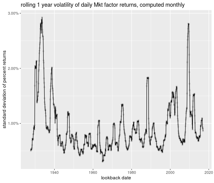
plot of chunk trun_testing
Now consider the running correlation of the “SMB” factor against the “Mkt” factor over time:
rho <- t_running_correlation(x = dff4$Mkt, y = dff4$SMB,
    time = index(dff4), window = 365.25, min_df = 180,
    lb_time = mo_ends)
library(ggplot2)
library(scales)
ph <- cbind(data.frame(mo_ends), data.frame(rho)) %>%
    setNames(c("date", "rho")) %>%
    ggplot(aes(date, rho)) + geom_line() + geom_point(alpha = 0.1) +
    geom_hline(yintercept = 0, linetype = 2, alpha = 0.5) +
    labs(x = "lookback date", y = expression(rho),
        title = "Rolling 1 year correlation of daily SMB and Mkt factor returns, computed monthly")
print(ph)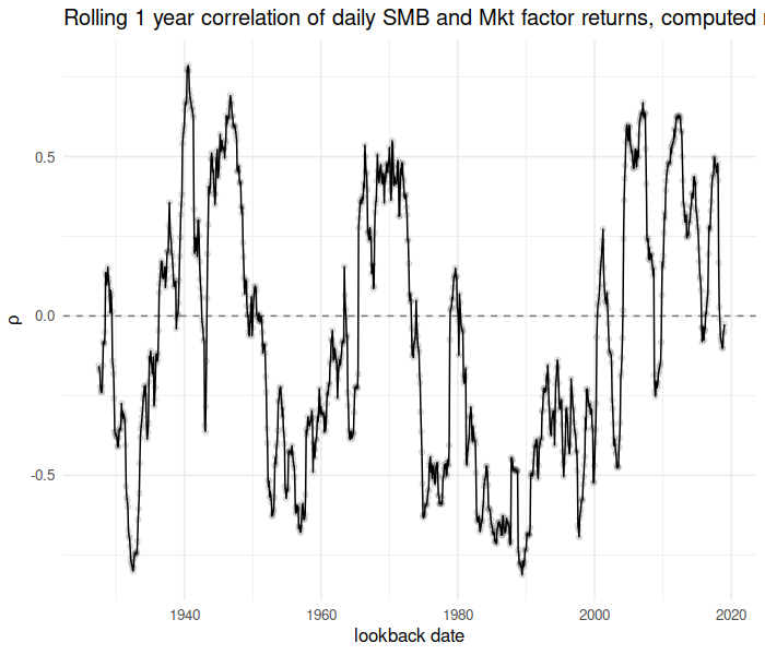
plot of chunk trun_corr_testing
We make every attempt to balance numerical robustness, computational efficiency and memory usage. As a bit of strawman-bashing, here we microbenchmark the running Z-score computation against the naive algorithm:
library(fromo)
library(moments)
library(microbenchmark)

set.seed(4422)
x <- rnorm(10000)

dumb_zscore <- function(x, window) {
    altz <- sapply(seq_along(x), function(iii) {
        rowi <- max(1, iii - window + 1)
        xrang <- x[rowi:iii]
        (x[iii] - mean(xrang))/sd(xrang)
    }, simplify = TRUE)
}

val1 <- running_zscored(x, 250)
val2 <- dumb_zscore(x, 250)
stopifnot(max(abs(val1 - val2), na.rm = TRUE) <= 1e-14)

microbenchmark(running_zscored(x, 250), dumb_zscore(x,
    250))
## Unit: microseconds
## expr min lq mean median uq max neval cld
## running_zscored(x, 250) 427 454 519 479 565 840 100 a
## dumb_zscore(x, 250) 173408 195446 219268 209673 227987 425059 100 bMore seriously, here we compare the running_sd3
function, which computes the standard deviation, mean and number of
elements with the roll_sd and roll_mean
functions from the roll package.
# dare I?
library(fromo)
library(microbenchmark)
library(roll)

set.seed(4422)
x <- rnorm(1e+05)
xm <- matrix(x)

v1 <- running_sd3(xm, 250)
rsd <- roll::roll_sd(xm, 250)
rmu <- roll::roll_mean(xm, 250)
# compute error on the 1000th row:
stopifnot(max(abs(v1[1000, ] - c(rsd[1000], rmu[1000],
    250))) < 1e-14)
# now timings:
microbenchmark(running_sd3(xm, 250), roll::roll_mean(xm,
    250), roll::roll_sd(xm, 250))
## Unit: microseconds
## expr min lq mean median uq max neval cld
## running_sd3(xm, 250) 5455 5638 5955 5753 5842 18177 100 a
## roll::roll_mean(xm, 250) 818 1025 1089 1052 1097 1931 100 b
## roll::roll_sd(xm, 250) 3327 3432 3661 3508 3601 16591 100 cOK, that’s not a fair comparison: roll_mean is optimized
to work columwise on a matrix. Let’s unbash this strawman. I create a
function using fromo::running_sd3 to compute a running mean
or running standard deviation columnwise on a matrix, then compare
that to roll_mean and roll_sd:
library(fromo)
library(microbenchmark)
library(roll)

set.seed(4422)
xm <- matrix(rnorm(4e+05), ncol = 100)
fromo_sd <- function(x, wins) {
    apply(x, 2, function(xc) {
        running_sd3(xc, wins)[, 1]
    })
}
fromo_mu <- function(x, wins) {
    apply(x, 2, function(xc) {
        running_sd3(xc, wins)[, 2]
    })
}
wins <- 1000
v1 <- fromo_sd(xm, wins)
rsd <- roll::roll_sd(xm, wins, min_obs = 3)

v2 <- fromo_mu(xm, wins)
rmu <- roll::roll_mean(xm, wins)
# compute error on the 2000th row:
stopifnot(max(abs(v1[2000, ] - rsd[2000, ])) < 1e-14)
stopifnot(max(abs(v2[2000, ] - rmu[2000, ])) < 1e-14)

# now timings: note fromo_mu and fromo_sd do
# exactly the same work, so only time one of them
microbenchmark(fromo_sd(xm, wins), roll::roll_mean(xm,
    wins), roll::roll_sd(xm, wins), times = 50L)
## Unit: milliseconds
## expr min lq mean median uq max neval cld
## fromo_sd(xm, wins) 43.6 44.4 47.7 46.8 48.3 61 50 a
## roll::roll_mean(xm, wins) 1.3 1.4 2.0 1.5 2.4 5 50 b
## roll::roll_sd(xm, wins) 3.5 3.6 4.6 3.9 4.7 13 50 cI suspect, however, that roll_mean is literally
recomputing moments over the entire window for every cell of the output,
instead of reusing computations, which fromo mostly
does:
library(roll)
library(microbenchmark)
set.seed(91823)
xm <- matrix(rnorm(2e+05), ncol = 10)
fromo_mu <- function(x, wins, ...) {
    apply(x, 2, function(xc) {
        running_sd3(xc, wins, ...)[, 2]
    })
}

microbenchmark(roll::roll_mean(xm, 10, min_obs = 3),
    roll::roll_mean(xm, 100, min_obs = 3), roll::roll_mean(xm,
        1000, min_obs = 3), roll::roll_mean(xm, 10000,
        min_obs = 3), fromo_mu(xm, 10, min_df = 3),
    fromo_mu(xm, 100, min_df = 3), fromo_mu(xm, 1000,
        min_df = 3), fromo_mu(xm, 10000, min_df = 3),
    times = 100L)
## Unit: microseconds
## expr min lq mean median uq max neval cld
## roll::roll_mean(xm, 10, min_obs = 3) 823 866 1121 909 1032 5444 100 a
## roll::roll_mean(xm, 100, min_obs = 3) 823 886 1030 941 990 4239 100 a
## roll::roll_mean(xm, 1000, min_obs = 3) 823 869 1085 924 970 7718 100 a
## roll::roll_mean(xm, 10000, min_obs = 3) 813 873 1041 909 947 4255 100 a
## fromo_mu(xm, 10, min_df = 3) 6746 6924 7961 7011 7633 20672 100 b
## fromo_mu(xm, 100, min_df = 3) 8553 8763 9938 8932 11541 16519 100 b
## fromo_mu(xm, 1000, min_df = 3) 25729 26368 27494 26680 28197 41629 100 c
## fromo_mu(xm, 10000, min_df = 3) 107917 109834 113658 111135 112992 274406 100 dThe runtime for operations from roll grow with the
window size. The equivalent operations from fromo also
consume more time for longer windows. In theory they would be invariant
with respect to window size, but I coded them to ‘restart’ the
computation periodically for improved accuracy. The user has control
over how often this happens, in order to balance speed and accuracy.
Here I set that parameter very large to show that runtimes need not grow
with window size:
library(fromo)
library(microbenchmark)
set.seed(91823)
xm <- matrix(rnorm(2e+05), ncol = 10)
fromo_mu <- function(x, wins, ...) {
    apply(x, 2, function(xc) {
        running_sd3(xc, wins, ...)[, 2]
    })
}
rp <- 1L + nrow(xm)

microbenchmark(fromo_mu(xm, 10, min_df = 3, restart_period = rp),
    fromo_mu(xm, 100, min_df = 3, restart_period = rp),
    fromo_mu(xm, 1000, min_df = 3, restart_period = rp),
    fromo_mu(xm, 10000, min_df = 3, restart_period = rp),
    times = 100L)
## Unit: milliseconds
## expr min lq mean median uq max neval cld
## fromo_mu(xm, 10, min_df = 3, restart_period = rp) 6.3 6.7 10.2 11.1 11 19 100 a
## fromo_mu(xm, 100, min_df = 3, restart_period = rp) 6.2 6.6 9.6 10.9 11 15 100 ab
## fromo_mu(xm, 1000, min_df = 3, restart_period = rp) 6.3 6.5 9.2 8.4 11 16 100 b
## fromo_mu(xm, 10000, min_df = 3, restart_period = rp) 5.6 5.9 8.9 10.3 11 15 100 bHere are some more benchmarks, also against the
rollingWindow package, for running sums:
library(microbenchmark)
library(fromo)
library(RollingWindow)
library(roll)

set.seed(12345)
x <- rnorm(10000)
xm <- matrix(x)
wins <- 1000

# run fun on each wins sized window...
silly_fun <- function(x, wins, fun, ...) {
    xout <- rep(NA, length(x))
    for (iii in seq_along(x)) {
        xout[iii] <- fun(x[max(1, iii - wins + 1):iii],
            ...)
    }
    xout
}
vals <- list(running_sum(x, wins, na_rm = FALSE), RollingWindow::RollingSum(x,
    wins, na_method = "ignore"), roll::roll_sum(xm,
    wins), silly_fun(x, wins, sum, na.rm = FALSE))

# check all equal?
stopifnot(max(unlist(lapply(vals[2:length(vals)], function(av) {
    err <- vals[[1]] - av
    max(abs(err[wins:length(err)]), na.rm = TRUE)
}))) < 1e-12)

# benchmark it
microbenchmark(running_sum(x, wins, na_rm = FALSE),
    RollingWindow::RollingSum(x, wins), running_sum(x,
        wins, na_rm = TRUE), RollingWindow::RollingSum(x,
        wins, na_method = "ignore"), roll::roll_sum(xm,
        wins))
## Unit: microseconds
## expr min lq mean median uq max neval cld
## running_sum(x, wins, na_rm = FALSE) 99 101 116 105 131 166 100 a
## RollingWindow::RollingSum(x, wins) 119 124 195 169 245 391 100 b
## running_sum(x, wins, na_rm = TRUE) 98 100 118 107 131 250 100 a
## RollingWindow::RollingSum(x, wins, na_method = "ignore") 262 270 408 366 499 796 100 c
## roll::roll_sum(xm, wins) 78 93 131 116 150 331 100 aAnd running means:
library(microbenchmark)
library(fromo)
library(RollingWindow)
library(roll)

set.seed(12345)
x <- rnorm(10000)
xm <- matrix(x)
wins <- 1000

vals <- list(running_mean(x, wins, na_rm = FALSE),
    RollingWindow::RollingMean(x, wins, na_method = "ignore"),
    roll::roll_mean(xm, wins), silly_fun(x, wins, mean,
        na.rm = FALSE))

# check all equal?
stopifnot(max(unlist(lapply(vals[2:length(vals)], function(av) {
    err <- vals[[1]] - av
    max(abs(err[wins:length(err)]), na.rm = TRUE)
}))) < 1e-12)

# benchmark it:
microbenchmark(running_mean(x, wins, na_rm = FALSE,
    restart_period = 1e+05), RollingWindow::RollingMean(x,
    wins), running_mean(x, wins, na_rm = TRUE, restart_period = 1e+05),
    RollingWindow::RollingMean(x, wins, na_method = "ignore"),
    roll::roll_mean(xm, wins))
## Unit: microseconds
## expr min lq mean median uq max neval cld
## running_mean(x, wins, na_rm = FALSE, restart_period = 1e+05) 96 99 113 102 125 188 100 a
## RollingWindow::RollingMean(x, wins) 121 125 189 170 241 383 100 b
## running_mean(x, wins, na_rm = TRUE, restart_period = 1e+05) 96 99 114 102 126 206 100 a
## RollingWindow::RollingMean(x, wins, na_method = "ignore") 260 268 373 371 465 618 100 c
## roll::roll_mean(xm, wins) 93 101 132 123 150 301 100 a