![]()

![]()
![]()
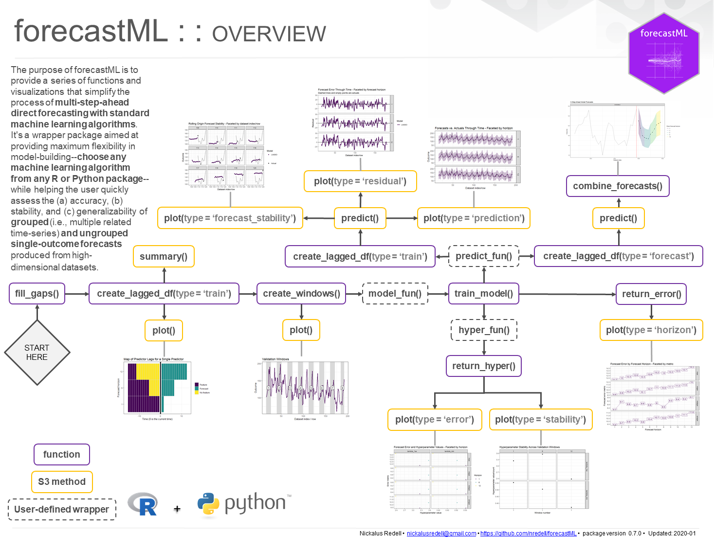
The purpose of forecastML is to provide a series of
functions and visualizations that simplify the process of
multi-step-ahead forecasting with standard machine learning
algorithms. It’s a wrapper package aimed at providing maximum
flexibility in model-building–choose any machine learning
algorithm from any R or Python
package–while helping the user quickly assess the (a) accuracy,
(b) stability, and (c) generalizability of grouped (i.e., multiple
related time series) and ungrouped forecasts produced from potentially
high-dimensional modeling datasets.
This package is inspired by Bergmeir, Hyndman, and Koo’s 2018 paper A note on the validity of cross-validation for evaluating autoregressive time series prediction. which supports–under certain conditions–forecasting with high-dimensional ML models without having to use methods that are time series specific.
The following quote from Bergmeir et al.’s article nicely sums up the aim of this package:
“When purely (non-linear, nonparametric) autoregressive methods are applied to forecasting problems, as is often the case (e.g., when using Machine Learning methods), the aforementioned problems of CV are largely irrelevant, and CV can and should be used without modification, as in the independent case.”
Forecasting with Python - scikit-learn in parallel (coming soon)
User-contributed notebooks welcome!
library(forecastML)
library(glmnet)
data("data_seatbelts", package = "forecastML")
data_train <- forecastML::create_lagged_df(data_seatbelts, type = "train", method = "direct",
outcome_col = 1, lookback = 1:15, horizon = 1:12)
windows <- forecastML::create_windows(data_train, window_length = 0)
model_fun <- function(data) {
x <- as.matrix(data[, -1, drop = FALSE])
y <- as.matrix(data[, 1, drop = FALSE])
model <- glmnet::cv.glmnet(x, y)
}
model_results <- forecastML::train_model(data_train, windows, model_name = "LASSO", model_function = model_fun)
prediction_fun <- function(model, data_features) {
data_pred <- data.frame("y_pred" = predict(model, as.matrix(data_features)),
"y_pred_lower" = predict(model, as.matrix(data_features)) - 30,
"y_pred_upper" = predict(model, as.matrix(data_features)) + 30)
}
data_forecast <- forecastML::create_lagged_df(data_seatbelts, type = "forecast", method = "direct",
outcome_col = 1, lookback = 1:15, horizon = 1:12)
data_forecasts <- predict(model_results, prediction_function = list(prediction_fun), data = data_forecast)
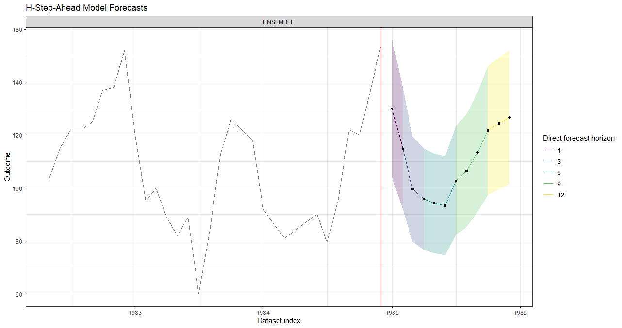
data_forecasts <- forecastML::combine_forecasts(data_forecasts)
plot(data_forecasts, data_actual = data_seatbelts[-(1:100), ], actual_indices = (1:nrow(data_seatbelts))[-(1:100)])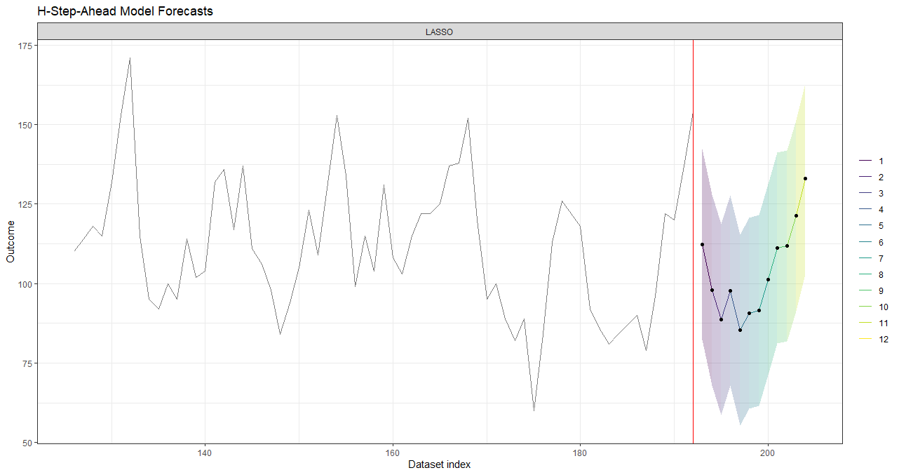
install.packages("forecastML")
library(forecastML)remotes::install_github("nredell/forecastML")
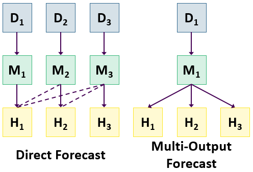
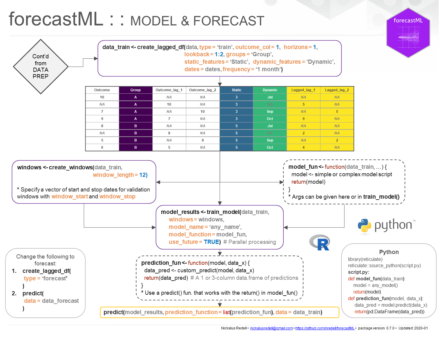
library(forecastML)The direct forecasting approach used in forecastML
involves the following steps:
1. Build a series of horizon-specific short-, medium-, and long-term forecast models.
2. Assess model generalization performance across a variety of heldout datasets through time.
3. Select those models that consistently performed the best at each forecast horizon and combine them to produce a single ensemble forecast.
Below is a plot of 5 forecast models used to produce a single 12-step-ahead forecast where each color represents a distinct horizon-specific ML model. From left to right these models are:
1: A feed-forward neural network (purple); 2: An ensemble of ML models; 3: A boosted tree model; 4: A LASSO regression model; 5: A LASSO regression model (yellow).
The multi-output forecasting approach used in forecastML
involves the following steps:
1. Build a single multi-output model that simultaneously forecasts over both short- and long-term forecast horizons.
2. Assess model generalization performance across a variety of heldout datasets through time.
3. Select the hyperparamters that minimize forecast error over all the relevant forecast horizons and re-train.
The main functions covered in each vignette are shown below as
function().
Detailed forecastML
overview vignette. create_lagged_df(),
create_windows(), train_model(),
return_error(), return_hyper(),
combine_forecasts()
Creating
custom feature lags for model training.
create_lagged_df(lookback_control = ...)
Direct
Forecasting with multiple or grouped time series.
fill_gaps(),
create_lagged_df(dates = ..., dynamic_features = ..., groups = ..., static_features = ...),
create_windows(), train_model(),
combine_forecasts()
Direct
Forecasting with multiple or grouped time series -
Sequences. fill_gaps(),
create_lagged_df(dates = ..., dynamic_features = ..., groups = ..., static_features = ...),
create_windows(), train_model(),
combine_forecasts()
Customizing
the user-defined wrapper functions. train()
and predict()
Forecast
combinations. combine_forecasts()
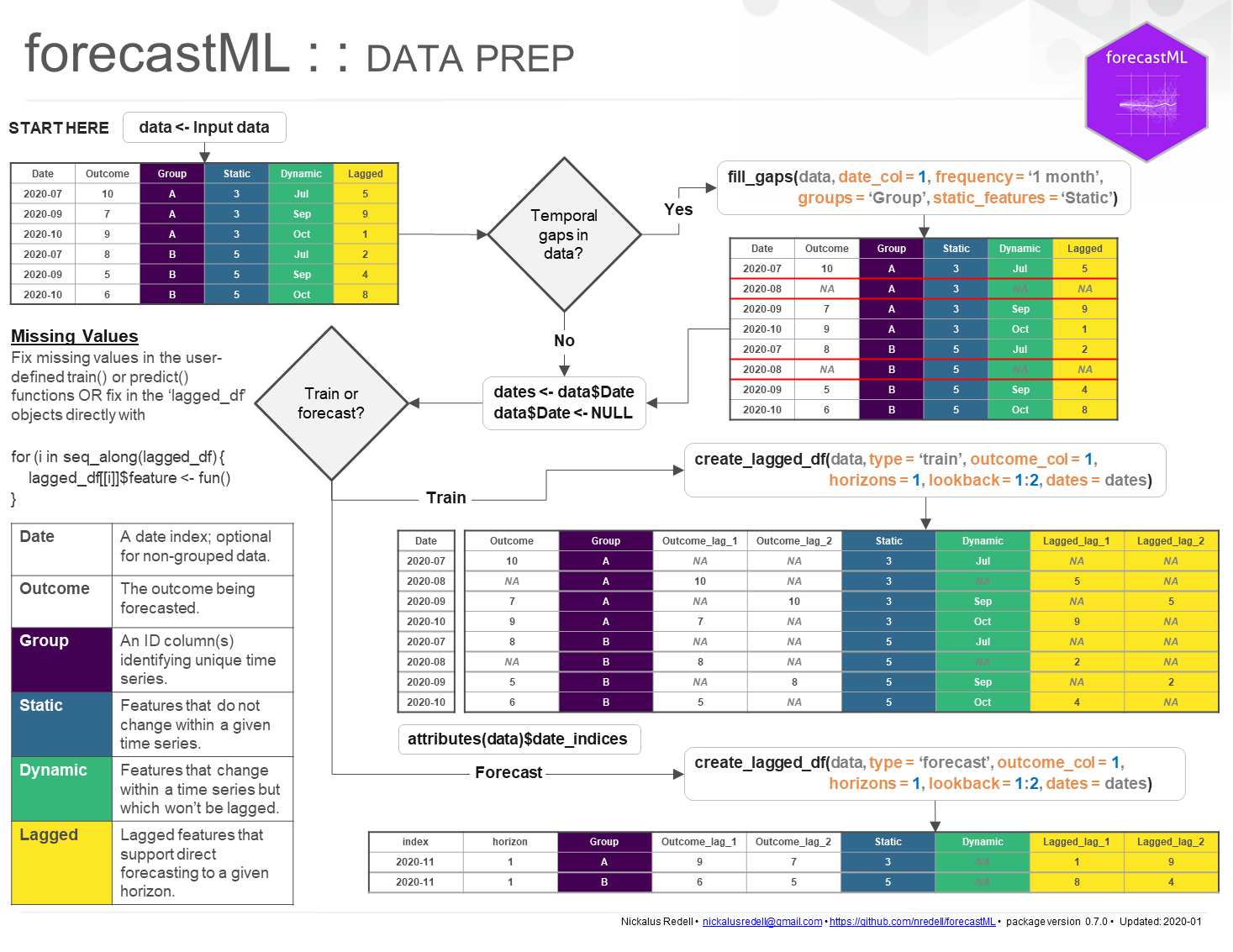
fill_gaps: Optional if no temporal
gaps/missing rows in data collection. Fill gaps in data collection and
prepare a dataset of evenly-spaced time series for modeling with lagged
features. Returns a ‘data.frame’ with missing rows added in so that you
can either (a) impute, remove, or ignore NAs prior to the
forecastML pipeline or (b) impute, remove, or ignore them
in the user-defined modeling function–depending on the NA
handling capabilities of the user-specified model.
create_lagged_df: Create model
training and forecasting datasets with lagged, grouped, dynamic, and
static features.
create_windows: Create
time-contiguous validation datasets for model evaluation.
train_model: Train the user-defined
model across forecast horizons and validation datasets.
return_error: Compute forecast
error across forecast horizons and validation datasets.
return_hyper: Return user-defined
model hyperparameters across validation datasets.
combine_forecasts: Combine multiple
horizon-specific forecast models to produce one forecast.
Q: Where does forecastML fit in
with respect to popular R machine learning packages like mlr3 and caret?
A: The idea is that forecastML
takes care of the tedious parts of forecasting with ML methods: creating
training and forecasting datasets with different types of
features–grouped, static, and dynamic–as well as simplifying validation
dataset creation to assess model performance at specific points in time.
That said, the workflow for packages like mlr3 and
caret would mostly occur inside of the user-supplied
modeling function which is passed into
forecastML::train_model(). Refer to the wrapper function
customization vignette for more details.
Q: How do I get the model training and
forecasting datasets as well as the trained models out of the
forecastML pipeline?
A: After running
forecastML::create_lagged_df() with either
type = "train" or type = "forecast", the
data.frames can be accessed with
my_lagged_df$horizon_h where “h” is an integer marking the
horizon-specific dataset (e.g., the value(s) passed in
horizons = ...). The trained models from
forecastML::train_model() can be accessed with
my_trained_model$horizon_h$window_w$model where “w” is the
validation window number from
forecastML::create_windows().
Below is an example of how to create 12 horizon-specific ML models to
forecast the number of DriversKilled 12 time periods into
the future using the Seatbelts dataset. Notice in the last
plot that there are multiple forecasts; these are from the slightly
different LASSO models trained in the nested cross-validation. An
example of selecting optimal hyperparameters and retraining to create a
single forecast model (i.e.,
create_windows(..., window_length = 0)) can be found in the
overview vignette.
library(glmnet)
library(forecastML)
# Sampled Seatbelts data from the R package datasets.
data("data_seatbelts", package = "forecastML")
# Example - Training data for 12 horizon-specific models w/ common lags per feature. The data do
# not have any missing rows or temporal gaps in data collection; if there were gaps,
# we would need to use fill_gaps() first.
horizons <- 1:12 # 12 models that forecast 1, 1:2, 1:3, ..., and 1:12 time steps ahead.
lookback <- 1:15 # A lookback of 1 to 15 dataset rows (1:15 * 'date frequency' if dates are given).
#------------------------------------------------------------------------------
# Create a dataset of lagged features for modeling.
data_train <- forecastML::create_lagged_df(data_seatbelts, type = "train",
outcome_col = 1, lookback = lookback,
horizon = horizons)
#------------------------------------------------------------------------------
# Create validation datasets for outer-loop nested cross-validation.
windows <- forecastML::create_windows(data_train, window_length = 12)
#------------------------------------------------------------------------------
# User-define model - LASSO
# A user-defined wrapper function for model training that takes the following
# arguments: (1) a horizon-specific data.frame made with create_lagged_df(..., type = "train")
# (e.g., my_lagged_df$horizon_h) and, optionally, (2) any number of additional named arguments
# which can also be passed in '...' in train_model(). The function returns a model object suitable for
# the user-defined predict function. The returned model may also be a list that holds meta-data such
# as hyperparameter settings.
model_function <- function(data, my_outcome_col) { # my_outcome_col = 1 could be defined here.
x <- data[, -(my_outcome_col), drop = FALSE]
y <- data[, my_outcome_col, drop = FALSE]
x <- as.matrix(x, ncol = ncol(x))
y <- as.matrix(y, ncol = ncol(y))
model <- glmnet::cv.glmnet(x, y)
return(model) # This model is the first argument in the user-defined predict() function below.
}
#------------------------------------------------------------------------------
# Train a model across forecast horizons and validation datasets.
# my_outcome_col = 1 is passed in ... but could have been defined in the user-defined model function.
model_results <- forecastML::train_model(data_train,
windows = windows,
model_name = "LASSO",
model_function = model_function,
my_outcome_col = 1, # ...
use_future = FALSE)
#------------------------------------------------------------------------------
# User-defined prediction function - LASSO
# The predict() wrapper function takes 2 positional arguments. First,
# the returned model from the user-defined modeling function (model_function() above).
# Second, a data.frame of model features. If predicting on validation data, expect the input data to be
# passed in the same format as returned by create_lagged_df(type = 'train') but with the outcome column
# removed. If forecasting, expect the input data to be in the same format as returned by
# create_lagged_df(type = 'forecast') but with the 'index' and 'horizon' columns removed. The function
# can return a 1- or 3-column data.frame with either (a) point
# forecasts or (b) point forecasts plus lower and upper forecast bounds (column order and names do not matter).
prediction_function <- function(model, data_features) {
x <- as.matrix(data_features, ncol = ncol(data_features))
data_pred <- data.frame("y_pred" = predict(model, x, s = "lambda.min"), # 1 column is required.
"y_pred_lower" = predict(model, x, s = "lambda.min") - 50, # optional.
"y_pred_upper" = predict(model, x, s = "lambda.min") + 50) # optional.
return(data_pred)
}
# Predict on the validation datasets.
data_valid <- predict(model_results, prediction_function = list(prediction_function), data = data_train)
#------------------------------------------------------------------------------
# Plot forecasts for each validation dataset.
plot(data_valid, horizons = c(1, 6, 12))
#------------------------------------------------------------------------------
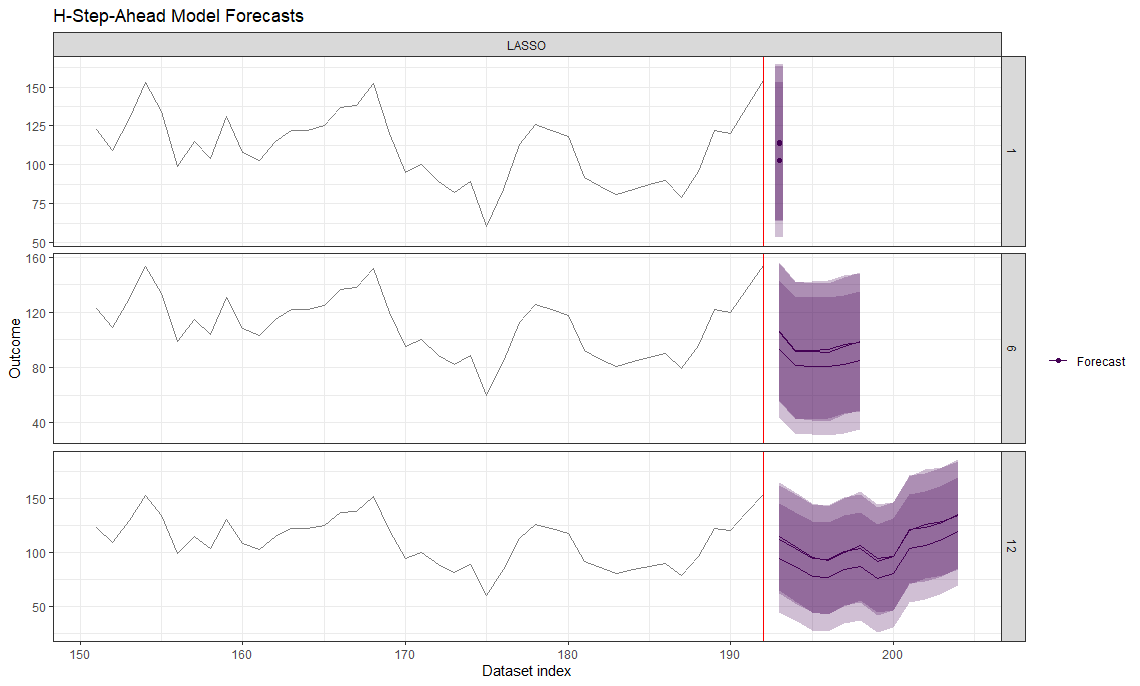
# Forecast.
# Forward-looking forecast data.frame.
data_forecast <- forecastML::create_lagged_df(data_seatbelts, type = "forecast",
outcome_col = 1, lookback = lookback, horizons = horizons)
# Forecasts.
data_forecasts <- predict(model_results, prediction_function = list(prediction_function), data = data_forecast)
# We'll plot a background dataset of actuals as well.
plot(data_forecasts,
data_actual = data_seatbelts[-(1:150), ],
actual_indices = as.numeric(row.names(data_seatbelts[-(1:150), ])),
horizons = c(1, 6, 12), windows = c(5, 10, 15))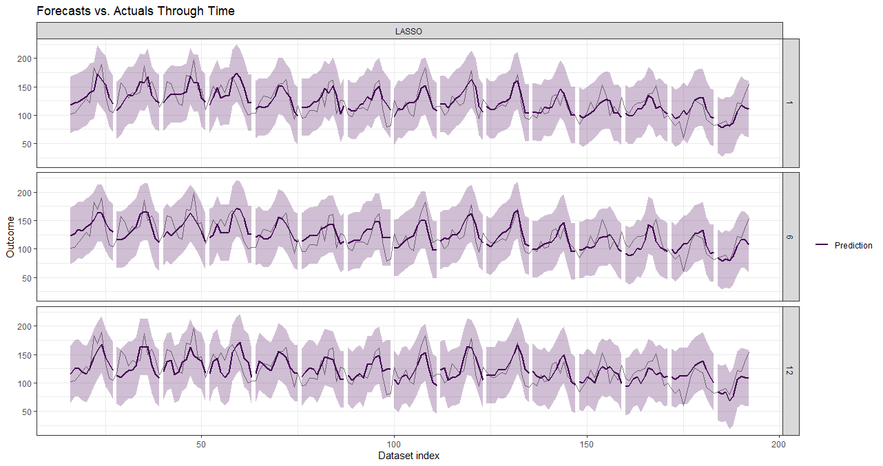
Now we’ll look at an example similar to above. The main difference is
that our user-defined modeling and prediction functions are now written
in Python. Thanks to the reticulate
R package, entire ML workflows already written in
Python can be imported into forecastML with
the simple addition of 2 lines of R code.
reticulate::source_python() function will run a .py
file and import any objects into your R environment. As
we’ll see below, we’ll only be importing library calls and functions to
keep our R environment clean.library(forecastML)
library(reticulate) # Move Python objects in and out of R. See the reticulate package for setup info.
reticulate::source_python("modeling_script.py") # Run a Python file and import objects into R.forecastML setup
for the seatbelt forecasting problem from the previous example.data("data_seatbelts", package = "forecastML")
horizons <- c(1, 12) # 2 models that forecast 1 and 1:12 time steps ahead.
# A lookback across select time steps in the past. Feature lags 1 through 9 will be silently dropped from the 12-step-ahead model.
lookback <- c(1, 3, 6, 9, 12, 15)
date_frequency <- "1 month" # Time step frequency.
# The date indices, which don't come with the stock dataset, should not be included in the modeling data.frame.
dates <- seq(as.Date("1969-01-01"), as.Date("1984-12-01"), by = date_frequency)
# Create a dataset of features for modeling.
data_train <- forecastML::create_lagged_df(data_seatbelts, type = "train", outcome_col = 1,
lookback = lookback, horizon = horizons,
dates = dates, frequency = date_frequency)
# Create 2 custom validation datasets for outer-loop nested cross-validation. The purpose of
# the multiple validation windows is to assess expected forecast accuracy for specific
# time periods while supporting an investigation of the hyperparameter stability for
# models trained on different time periods. Validation windows can overlap.
window_start <- c(as.Date("1983-01-01"), as.Date("1984-01-01"))
window_stop <- c(as.Date("1983-12-01"), as.Date("1984-12-01"))
windows <- forecastML::create_windows(data_train, window_start = window_start, window_stop = window_stop)Python modeling file
that we source()’d above. The Python wrapper function
inputs and returns for py_model_function() and
py_prediction_function() are the same as their
R counterparts. Just be sure to expect and return
pandas DataFrames as conversion from
numpy arrays has not been tested.
import pandas as pd
from sklearn import linear_model
from sklearn.preprocessing import StandardScaler

# User-defined model.
# A user-defined wrapper function for model training that takes the following
# arguments: (1) a horizon-specific pandas DataFrame made with create_lagged_df(..., type = "train")
# (e.g., my_lagged_df$horizon_h)
def py_model_function(data):

  X = data.iloc[:, 1:]
  y = data.iloc[:, 0]

  scaler = StandardScaler()
  X = scaler.fit_transform(X)

  model_lasso = linear_model.Lasso(alpha = 0.1)

  model_lasso.fit(X = X, y = y)

  return({'model': model_lasso, 'scaler': scaler})

# User-defined prediction function.
# The predict() wrapper function takes 2 positional arguments. First,
# the returned model from the user-defined modeling function (py_model_function() above).
# Second, a pandas DataFrame of model features. For numeric outcomes, the function
# can return a 1- or 3-column pandas DataFrame with either (a) point
# forecasts or (b) point forecasts plus lower and upper forecast bounds (column order and names do not matter).
def py_prediction_function(model_list, data_x):

  data_x = model_list['scaler'].transform(data_x)

  data_pred = pd.DataFrame({'y_pred': model_list['model'].predict(data_x)})

return(data_pred)Python wrapper functions.# Train a model across forecast horizons and validation datasets.
model_results <- forecastML::train_model(data_train,
windows = windows,
model_name = "LASSO",
model_function = py_model_function,
use_future = FALSE)
# Predict on the validation datasets.
data_valid <- predict(model_results, prediction_function = list(py_prediction_function), data = data_train)
# Plot forecasts for each validation dataset.
plot(data_valid, horizons = c(1, 12))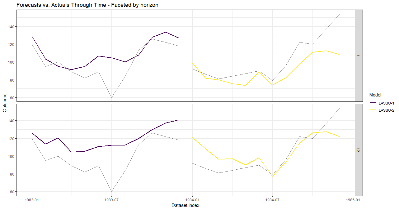
Python wrapper
functions. The final wrapper functions may eventually have fixed
hyperparameters or complicated model ensembles based on repeated model
training and investigation.# Forward-looking forecast data.frame.
data_forecast <- forecastML::create_lagged_df(data_seatbelts, type = "forecast", outcome_col = 1,
lookback = lookback, horizon = horizons,
dates = dates, frequency = date_frequency)
# Forecasts.
data_forecasts <- predict(model_results, prediction_function = list(py_prediction_function),
data = data_forecast)
# We'll plot a background dataset of actuals as well.
plot(data_forecasts, data_actual = data_seatbelts[-(1:150), ],
actual_indices = dates[-(1:150)], horizons = c(1, 12))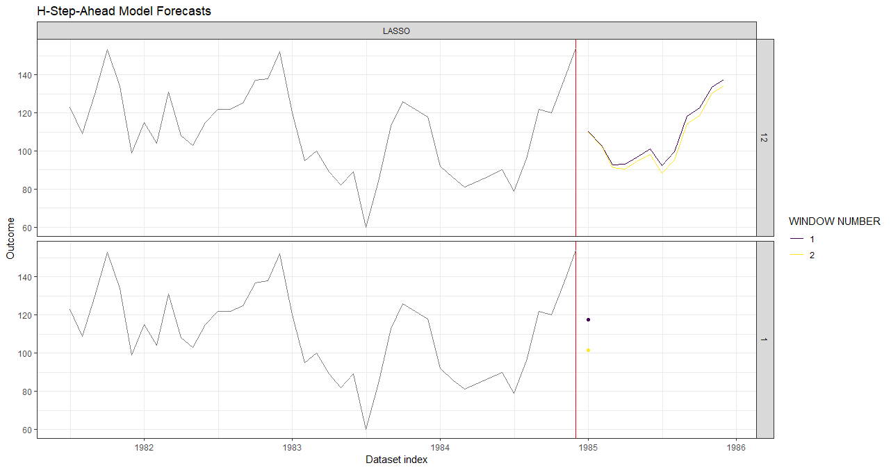
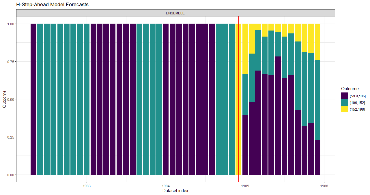
This is the same seatbelt dataset example except now, instead of 1 model for each forecast horizon, we’ll build 1 multi-output neural network model that forecasts 12 steps into the future.
Given that this is a small dataset, the multi-output approach would require a decent amount of tuning to produce accurate results. An alternative would be to forecast, say, horizons 6 through 12 if longer term forecasts were of interest to reduce the number of parameters; the output neurons do not have to start at a horizon of 1 or even be contiguous.
library(forecastML)
library(keras)  # Using the TensorFlow 2.0 backend.

data("data_seatbelts", package = "forecastML")

data_seatbelts[] <- lapply(data_seatbelts, function(x) {
  (x - mean(x, na.rm = TRUE)) / sd(x, na.rm = TRUE)
})

date_frequency <- "1 month"
dates <- seq(as.Date("1969-01-01"), as.Date("1984-12-01"), by = date_frequency)

data_train <- forecastML::create_lagged_df(data_seatbelts, type = "train", method = "multi_output",
                                           outcome_col = 1, lookback = 1:15, horizons = 1:12,
                                           dates = dates, frequency = date_frequency,
                                           dynamic_features = "law")

# 'window_length = 0' creates 1 historical training dataset with no external validation datasets.
# Set it to, say, 24 to see the model and forecast stability when trained across different slices
# of historical data.
windows <- forecastML::create_windows(data_train, window_length = 0)

#------------------------------------------------------------------------------
# 'data_y' consists of 1 column for each forecast horizon--here, 12.
model_fun <- function(data, horizons) {  # 'horizons' is passed in train_model().

  data_x <- apply(as.matrix(data[, -(1:length(horizons))]), 2, function(x){ifelse(is.na(x), 0, x)})
  data_y <- apply(as.matrix(data[, 1:length(horizons)]), 2, function(x){ifelse(is.na(x), 0, x)})

  layers_x_input <- keras::layer_input(shape = ncol(data_x))

  layers_x_output <- layers_x_input %>%
    keras::layer_dense(ncol(data_x), activation = "relu") %>%
    keras::layer_dense(ncol(data_x), activation = "relu") %>%
    keras::layer_dense(length(horizons))

  model <- keras::keras_model(inputs = layers_x_input, outputs = layers_x_output) %>%
    keras::compile(optimizer = 'adam', loss = 'mean_absolute_error')

  early_stopping <- callback_early_stopping(monitor = 'val_loss', patience = 2)

  tensorflow::tf$random$set_seed(224)

  model_results <- model %>%
    keras::fit(x = list(as.matrix(data_x)), y = list(as.matrix(data_y)),
               validation_split = 0.2, callbacks = c(early_stopping), verbose = FALSE)

  return(list("model" = model, "model_results" = model_results))
}
#------------------------------------------------------------------------------
# The predict() wrapper function will return a data.frame with a number of columns
# equaling the number of forecast horizons.
prediction_fun <- function(model, data_features) {

  data_features[] <- lapply(data_features, function(x){ifelse(is.na(x), 0, x)})
  data_features <- list(as.matrix(data_features, ncol = ncol(data_features)))

  data_pred <- data.frame(predict(model$model, data_features))
  names(data_pred) <- paste0("y_pred_", 1:ncol(data_pred))

  return(data_pred)
}
#------------------------------------------------------------------------------

model_results <- forecastML::train_model(data_train, windows, model_name = "Multi-Output NN",
                                         model_function = model_fun,
                                         horizons = 1:12)

data_valid <- predict(model_results, prediction_function = list(prediction_fun), data = data_train)

# We'll plot select forecast horizons to reduce visual clutter.
plot(data_valid, facet = ~ model, horizons = c(1, 3, 6, 12))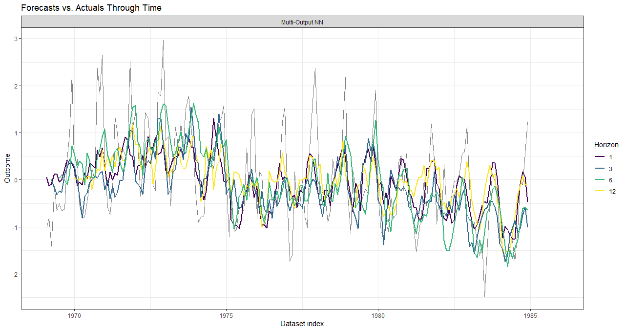
combine_forecasts() aren’t
necessary as we’ve trained only 1 model.data_forecast <- forecastML::create_lagged_df(data_seatbelts, type = "forecast", method = "multi_output",
outcome_col = 1, lookback = 1:15, horizons = 1:12,
dates = dates, frequency = date_frequency,
dynamic_features = "law")
data_forecasts <- predict(model_results, prediction_function = list(prediction_fun), data = data_forecast)
plot(data_forecasts, facet = NULL, data_actual = data_seatbelts[-(1:100), ], actual_indices = dates[-(1:100)])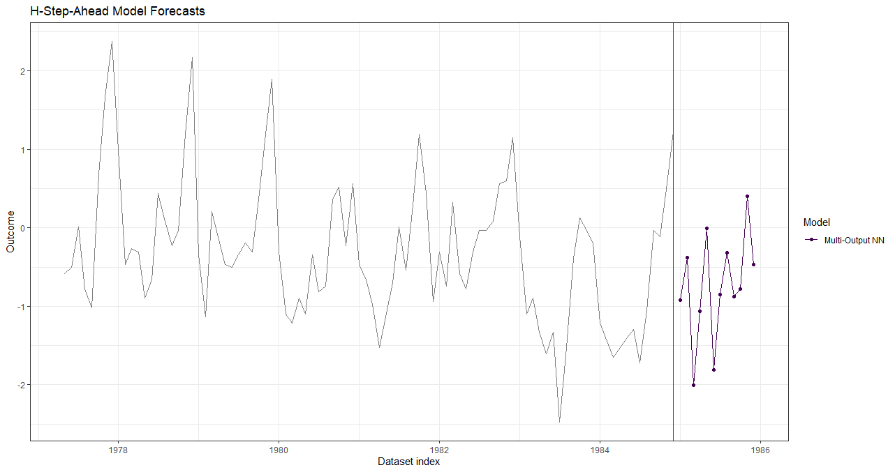
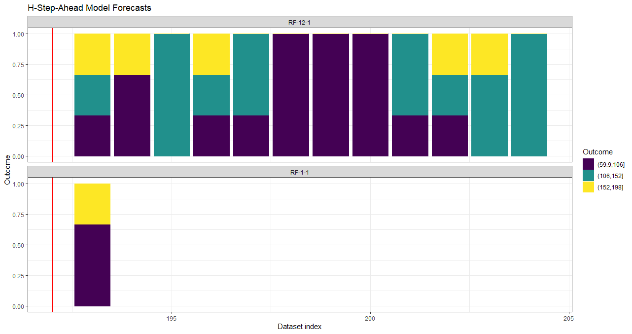
data("data_seatbelts", package = "forecastML")

# Create an artifical factor outcome for illustration' sake.
data_seatbelts$DriversKilled <- cut(data_seatbelts$DriversKilled, 3)

horizons <- c(1, 12)  # 2 models that forecast 1 and 1:12 time steps ahead.

# A lookback across select time steps in the past. Feature lag 1 will be silently dropped from the 12-step-ahead model.
lookback <- c(1, 12, 18)

date_frequency <- "1 month"  # Time step frequency.

# The date indices, which don't come with the stock dataset, should not be included in the modeling data.frame.
dates <- seq(as.Date("1969-01-01"), as.Date("1984-12-01"), by = date_frequency)

# Create a dataset of features for modeling.
data_train <- forecastML::create_lagged_df(data_seatbelts, type = "train", outcome_col = 1,
                                           lookback = lookback, horizon = horizons,
                                           dates = dates, frequency = date_frequency)

# We won't use nested cross-validation; rather, we'll train a model over the entire training dataset.
windows <- forecastML::create_windows(data_train, window_length = 0)

# This is the model-training dataset.
plot(windows, data_train)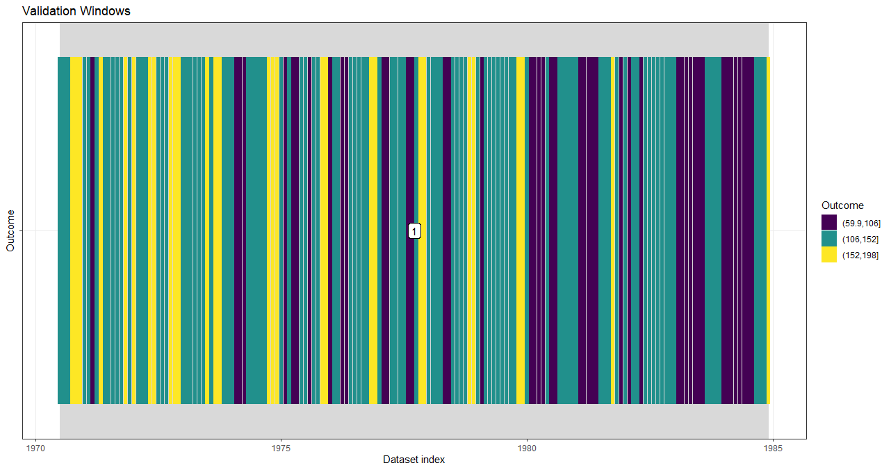
model_function <- function(data, my_outcome_col) {  # my_outcome_col = 1 could be defined here.

  outcome_names <- names(data)[1]
  model_formula <- formula(paste0(outcome_names,  "~ ."))

  set.seed(224)
  model <- randomForest::randomForest(formula = model_formula, data = data, ntree = 3)
  return(model)  # This model is the first argument in the user-defined predict() function below.
}

#------------------------------------------------------------------------------
# Train a model across forecast horizons and validation datasets.
# my_outcome_col = 1 is passed in ... but could have been defined in the user-defined model function.
model_results <- forecastML::train_model(data_train,
                                         windows = windows,
                                         model_name = "RF",
                                         model_function = model_function,
                                         my_outcome_col = 1,  # ...
                                         use_future = FALSE)

#------------------------------------------------------------------------------
# User-defined prediction function.
#
# The predict() wrapper function takes 2 positional arguments. First,
# the returned model from the user-defined modeling function (model_function() above).
# Second, a data.frame of model features. If predicting on validation data, expect the input data to be
# passed in the same format as returned by create_lagged_df(type = 'train') but with the outcome column
# removed. If forecasting, expect the input data to be in the same format as returned by
# create_lagged_df(type = 'forecast') but with the 'index' and 'horizon' columns removed.
#
# For factor outcomes, the function can return either (a) a 1-column data.frame with factor level
# predictions or (b) an L-column data.frame of predicted class probabilities where 'L' equals the
# number of levels in the outcome; the order of the return()'d columns should match the order of the
# outcome factor levels from left to right which is the default behavior of most predict() functions.

# Predict/forecast a single factor level.
prediction_function_level <- function(model, data_features) {

  data_pred <- data.frame("y_pred" = predict(model, data_features, type = "response"))

  return(data_pred)
}

# Predict/forecast outcome class probabilities.
prediction_function_prob <- function(model, data_features) {

  data_pred <- data.frame("y_pred" = predict(model, data_features, type = "prob"))

  return(data_pred)
}

# Predict on the validation datasets.
data_valid_level <- predict(model_results,
                            prediction_function = list(prediction_function_level),
                            data = data_train)
data_valid_prob <- predict(model_results,
                           prediction_function = list(prediction_function_prob),
                           data = data_train)
Predict historical factor levels.
With window_length = 0 these are essentially plots
of model fit.
plot(data_valid_level, horizons = c(1, 12))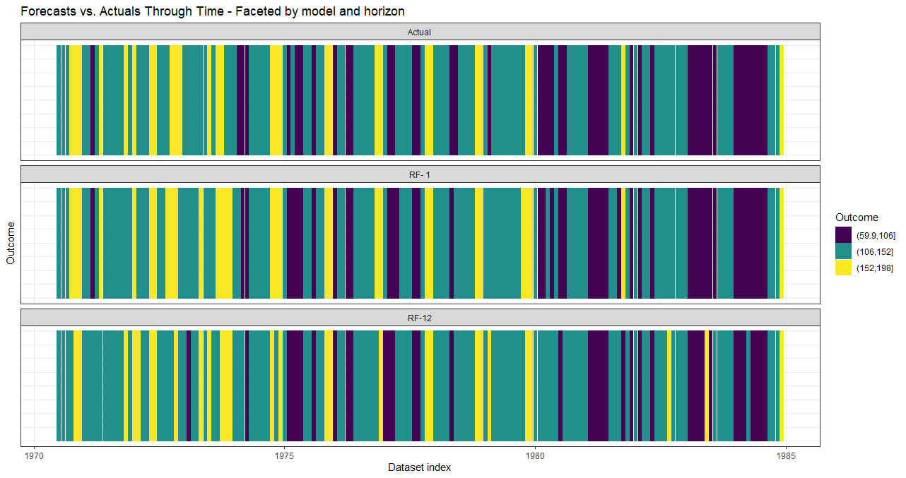
plot(data_valid_prob, horizons = c(1, 12))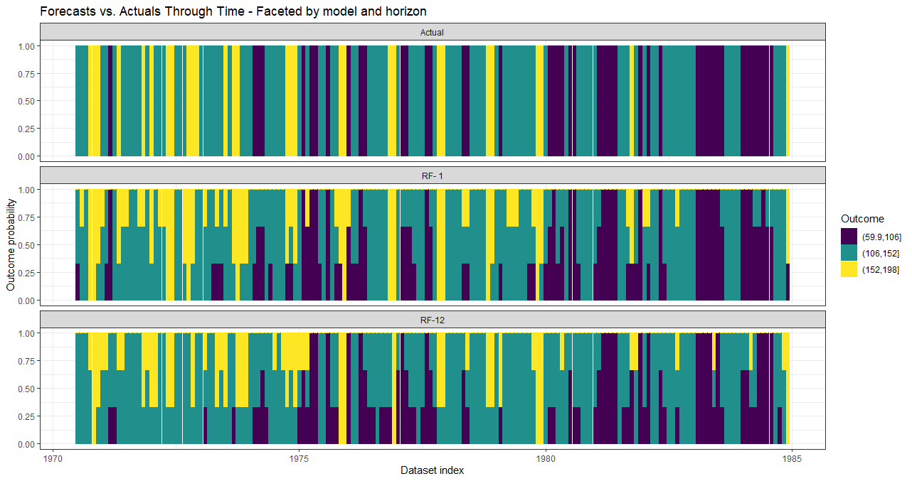
# Forward-looking forecast data.frame.
data_forecast <- forecastML::create_lagged_df(data_seatbelts, type = "forecast",
                                              outcome_col = 1, lookback = lookback, horizons = horizons)

# Forecasts.
data_forecasts_level <- predict(model_results,
                                prediction_function = list(prediction_function_level),
                                data = data_forecast)

data_forecasts_prob <- predict(model_results,
                                prediction_function = list(prediction_function_prob),
data = data_forecast)plot(data_forecasts_level)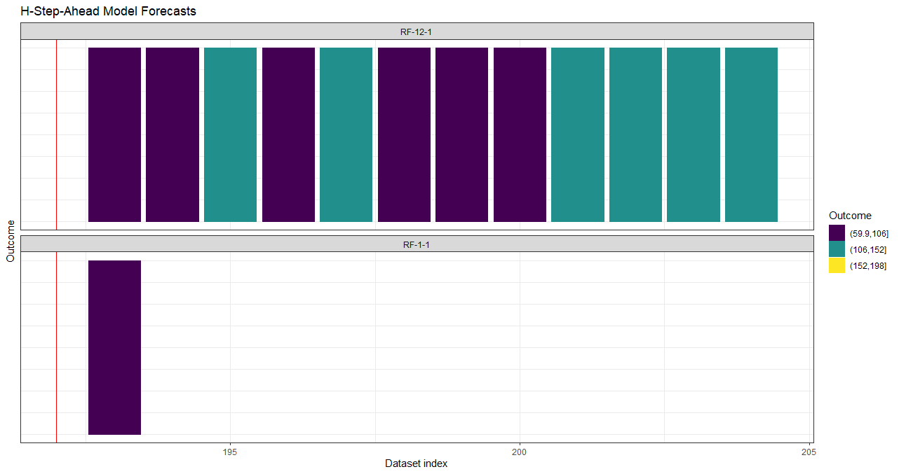
plot(data_forecasts_prob)