![]()
diffeqr is a package for solving differential equations in R. It utilizes DifferentialEquations.jl for its core routines to give high performance solving of ordinary differential equations (ODEs), stochastic differential equations (SDEs), delay differential equations (DDEs), and differential-algebraic equations (DAEs) directly in R.
If you have any questions, or just want to chat about solvers/using the package, please feel free to chat in the Zulip channel. For bug reports, feature requests, etc., please submit an issue.
diffeqr is registered into CRAN. Thus to add the package, use:
install.packages("diffeqr")To install the master branch of the package (for developers), use:
devtools::install_github('SciML/diffeqr', build_vignettes=T)Note that the first invocation of
diffeqr::diffeq_setup() will install both Julia and the
required packages if they are missing. If you wish to have it use an
existing Julia binary, make sure that julia is found in the
path. For more information see the julia_setup() function
from JuliaCall.
As a demonstration, check out the following notebooks:
diffeqr provides a direct wrapper over DifferentialEquations.jl. The namespace is setup so that the standard syntax of Julia translates directly over to the R environment. There are two things to keep in mind:
de$! are replaced with
_bang, for example solve! becomes
solve_bang.Let’s solve the linear ODE u'=1.01u. First setup the
package:
de <- diffeqr::diffeq_setup()Define the derivative function f(u,p,t).
f <- function(u,p,t) {
  return(1.01*u)
}
Then we give it an initial condition and a time span to solve over:
u0 <- 1/2
tspan <- c(0., 1.)
With those pieces we define the ODEProblem and
solve the ODE:
prob = de$ODEProblem(f, u0, tspan)
sol = de$solve(prob)
This gives back a solution object for which sol$t are
the time points and sol$u are the values. We can treat the
solution as a continuous object in time via
sol$.(0.2)and a high order interpolation will compute the value at
t=0.2. We can check the solution by plotting it:
plot(sol$t,sol$u,"l")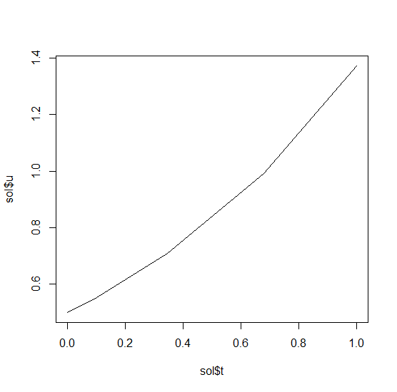
Now let’s solve the Lorenz equations. In this case, our initial condition is a vector and our derivative functions takes in the vector to return a vector (note: arbitrary dimensional arrays are allowed). We would define this as:
f <- function(u,p,t) {
  du1 = p[1]*(u[2]-u[1])
  du2 = u[1]*(p[2]-u[3]) - u[2]
  du3 = u[1]*u[2] - p[3]*u[3]
  return(c(du1,du2,du3))
}
Here we utilized the parameter array p. Thus we use
diffeqr::ode.solve like before, but also pass in parameters
this time:
u0 <- c(1.0,0.0,0.0)
tspan <- c(0.0,100.0)
p <- c(10.0,28.0,8/3)
prob <- de$ODEProblem(f, u0, tspan, p)
sol <- de$solve(prob)
The returned solution is like before except now sol$u is
an array of arrays, where sol$u[i] is the full system at
time sol$t[i]. It can be convenient to turn this into an R
matrix through sapply:
mat <- sapply(sol$u,identity)This has each row as a time series. t(mat) makes each
column a time series. It is sometimes convenient to turn the output into
a data.frame which is done via:
udf <- as.data.frame(t(mat))Now we can use matplot to plot the timeseries
together:
matplot(sol$t,udf,"l",col=1:3)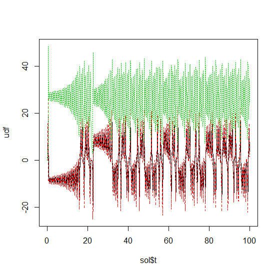
Now we can use the Plotly package to draw a phase plot:
plotly::plot_ly(udf, x = ~V1, y = ~V2, z = ~V3, type = 'scatter3d', mode = 'lines')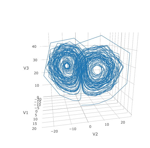
Plotly is much prettier!
If we want to have a more accurate solution, we can send
abstol and reltol. Defaults are
1e-6 and 1e-3 respectively. Generally you can
think of the digits of accuracy as related to 1 plus the exponent of the
relative tolerance, so the default is two digits of accuracy. Absolute
tolernace is the accuracy near 0.
In addition, we may want to choose to save at more time points. We do
this by giving an array of values to save at as saveat.
Together, this looks like:
abstol <- 1e-8
reltol <- 1e-8
saveat <- 0:10000/100
sol <- de$solve(prob,abstol=abstol,reltol=reltol,saveat=saveat)
udf <- as.data.frame(t(sapply(sol$u,identity)))
plotly::plot_ly(udf, x = ~V1, y = ~V2, z = ~V3, type = 'scatter3d', mode = 'lines')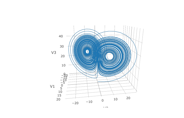
We can also choose to use a different algorithm. The choice is done using a string that matches the Julia syntax. See the ODE tutorial for details. The list of choices for ODEs can be found at the ODE Solvers page. For example, let’s use a 9th order method due to Verner:
sol <- de$solve(prob,de$Vern9(),abstol=abstol,reltol=reltol,saveat=saveat)Note that each algorithm choice will cause a JIT compilation.
One way to enhance the performance of your code is to define the
function in Julia so that way it is JIT compiled. diffeqr is built using
the JuliaCall
package, and so you can utilize the Julia JIT compiler. We expose
this automatically over ODE functions via jitoptimize_ode,
like in the following example:
f <- function(u,p,t) {
  du1 = p[1]*(u[2]-u[1])
  du2 = u[1]*(p[2]-u[3]) - u[2]
  du3 = u[1]*u[2] - p[3]*u[3]
  return(c(du1,du2,du3))
}
u0 <- c(1.0,0.0,0.0)
tspan <- c(0.0,100.0)
p <- c(10.0,28.0,8/3)
prob <- de$ODEProblem(f, u0, tspan, p)
fastprob <- diffeqr::jitoptimize_ode(de,prob)
sol <- de$solve(fastprob,de$Tsit5())
Note that the first evaluation of the function will have an ~2 second lag since the compiler will run, and all subsequent runs will be orders of magnitude faster than the pure R function. This means it’s great for expensive functions (ex. large PDEs) or functions called repeatedly, like during optimization of parameters.
We can also use the JuliaCall functions to directly define the function in Julia to eliminate the R interpreter overhead and get full JIT compilation:
julf <- JuliaCall::julia_eval("
function julf(du,u,p,t)
  du[1] = 10.0*(u[2]-u[1])
  du[2] = u[1]*(28.0-u[3]) - u[2]
  du[3] = u[1]*u[2] - (8/3)*u[3]
end")
JuliaCall::julia_assign("u0", u0)
JuliaCall::julia_assign("p", p)
JuliaCall::julia_assign("tspan", tspan)
prob3 = JuliaCall::julia_eval("ODEProblem(julf, u0, tspan, p)")
sol = de$solve(prob3,de$Tsit5())
To demonstrate the performance advantage, let’s time them all:
> system.time({ for (i in 1:100){ de$solve(prob    ,de$Tsit5()) }})
   user  system elapsed
   6.69    0.06    6.78
> system.time({ for (i in 1:100){ de$solve(fastprob,de$Tsit5()) }})
   user  system elapsed
   0.11    0.03    0.14
> system.time({ for (i in 1:100){ de$solve(prob3   ,de$Tsit5()) }})
   user  system elapsed
   0.14    0.02    0.15
This is about a 50x improvement!
Using Julia’s ModelingToolkit for tracing to JIT compile via Julia has a few known limitations:
cos and sin all fall into this
category. Notably, matrix multiplication is not supported.Solving stochastic differential equations (SDEs) is the similar to
ODEs. To solve an SDE, you use diffeqr::sde.solve and give
two functions: f and g, where
du = f(u,t)dt + g(u,t)dW_t
de <- diffeqr::diffeq_setup()
f <- function(u,p,t) {
  return(1.01*u)
}
g <- function(u,p,t) {
  return(0.87*u)
}
u0 <- 1/2
tspan <- c(0.0,1.0)
prob <- de$SDEProblem(f,g,u0,tspan)
sol <- de$solve(prob)
udf <- as.data.frame(t(sapply(sol$u,identity)))
plotly::plot_ly(udf, x = sol$t, y = sol$u, type = 'scatter', mode = 'lines')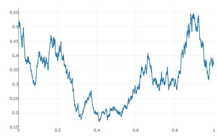
Let’s add diagonal multiplicative noise to the Lorenz attractor. diffeqr defaults to diagonal noise when a system of equations is given. This is a unique noise term per system variable. Thus we generalize our previous functions as follows:
f <- function(u,p,t) {
  du1 = p[1]*(u[2]-u[1])
  du2 = u[1]*(p[2]-u[3]) - u[2]
  du3 = u[1]*u[2] - p[3]*u[3]
  return(c(du1,du2,du3))
}
g <- function(u,p,t) {
  return(c(0.3*u[1],0.3*u[2],0.3*u[3]))
}
u0 <- c(1.0,0.0,0.0)
tspan <- c(0.0,1.0)
p <- c(10.0,28.0,8/3)
prob <- de$SDEProblem(f,g,u0,tspan,p)
sol <- de$solve(prob,saveat=0.005)
udf <- as.data.frame(t(sapply(sol$u,identity)))
plotly::plot_ly(udf, x = ~V1, y = ~V2, z = ~V3, type = 'scatter3d', mode = 'lines')
Using a JIT compiled function for the drift and diffusion functions can greatly enhance the speed here. With the speed increase we can comfortably solve over long time spans:
tspan <- c(0.0,100.0)
prob <- de$SDEProblem(f,g,u0,tspan,p)
fastprob <- diffeqr::jitoptimize_sde(de,prob)
sol <- de$solve(fastprob,saveat=0.005)
udf <- as.data.frame(t(sapply(sol$u,identity)))
plotly::plot_ly(udf, x = ~V1, y = ~V2, z = ~V3, type = 'scatter3d', mode = 'lines')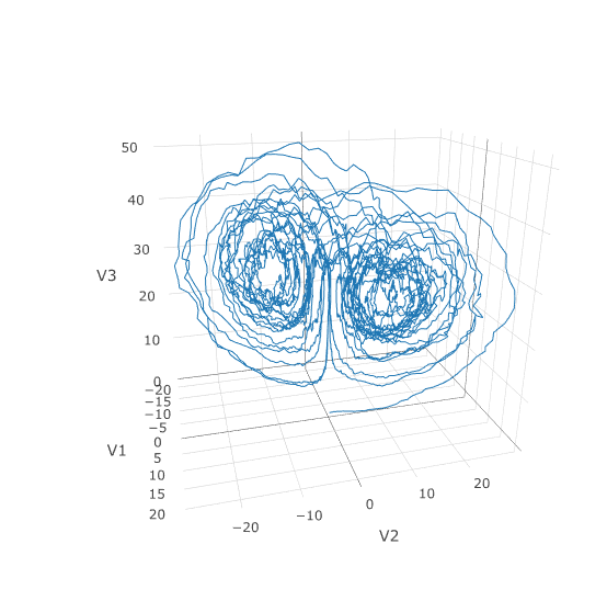
Let’s see how much faster the JIT-compiled version was:
> system.time({ for (i in 1:5){ de$solve(prob    ) }})
   user  system elapsed
 146.40    0.75  147.22
> system.time({ for (i in 1:5){ de$solve(fastprob) }})
   user  system elapsed
   1.07    0.10    1.17
Holy Monster’s Inc. that’s about 145x faster.
In many cases you may want to share noise terms across the system.
This is known as non-diagonal noise. The DifferentialEquations.jl
SDE Tutorial explains how the matrix form of the diffusion term
corresponds to the summation style of multiple Wiener processes.
Essentially, the row corresponds to which system the term is applied to,
and the column is which noise term. So du[i,j] is the
amount of noise due to the jth Wiener process that’s
applied to u[i]. We solve the Lorenz system with correlated
noise as follows:
f <- JuliaCall::julia_eval("
function f(du,u,p,t)
  du[1] = 10.0*(u[2]-u[1])
  du[2] = u[1]*(28.0-u[3]) - u[2]
  du[3] = u[1]*u[2] - (8/3)*u[3]
end")
g <- JuliaCall::julia_eval("
function g(du,u,p,t)
  du[1,1] = 0.3u[1]
  du[2,1] = 0.6u[1]
  du[3,1] = 0.2u[1]
  du[1,2] = 1.2u[2]
  du[2,2] = 0.2u[2]
  du[3,2] = 0.3u[2]
end")
u0 <- c(1.0,0.0,0.0)
tspan <- c(0.0,100.0)
noise_rate_prototype <- matrix(c(0.0,0.0,0.0,0.0,0.0,0.0), nrow = 3, ncol = 2)

JuliaCall::julia_assign("u0", u0)
JuliaCall::julia_assign("tspan", tspan)
JuliaCall::julia_assign("noise_rate_prototype", noise_rate_prototype)
prob <- JuliaCall::julia_eval("SDEProblem(f, g, u0, tspan, p, noise_rate_prototype=noise_rate_prototype)")
sol <- de$solve(prob)
udf <- as.data.frame(t(sapply(sol$u,identity)))
plotly::plot_ly(udf, x = ~V1, y = ~V2, z = ~V3, type = 'scatter3d', mode = 'lines')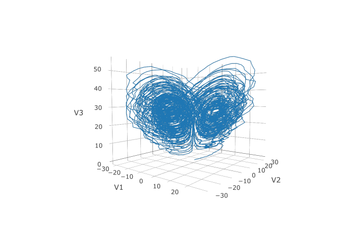
Here you can see that the warping effect of the noise correlations is quite visible! Note that we applied JIT compilation since it’s quite necessary for any difficult stochastic example.
A differential-algebraic equation is defined by an implicit function
f(du,u,p,t)=0. All of the controls are the same as the
other examples, except here you define a function which returns the
residuals for each part of the equation to define the DAE. The initial
value u0 and the initial derivative du0 are
required, though they do not necessarily have to satisfy f
(known as inconsistent initial conditions). The methods will
automatically find consistent initial conditions. In order for this to
occur, differential_vars must be set. This vector states
which of the variables are differential (have a derivative term), with
false meaning that the variable is purely algebraic.
This example shows how to solve the Robertson equation:
f <- function (du,u,p,t) {
  resid1 = - 0.04*u[1]              + 1e4*u[2]*u[3] - du[1]
  resid2 = + 0.04*u[1] - 3e7*u[2]^2 - 1e4*u[2]*u[3] - du[2]
  resid3 = u[1] + u[2] + u[3] - 1.0
  c(resid1,resid2,resid3)
}
u0 <- c(1.0, 0, 0)
du0 <- c(-0.04, 0.04, 0.0)
tspan <- c(0.0,100000.0)
differential_vars <- c(TRUE,TRUE,FALSE)
prob <- de$DAEProblem(f,du0,u0,tspan,differential_vars=differential_vars)
sol <- de$solve(prob)
udf <- as.data.frame(t(sapply(sol$u,identity)))
plotly::plot_ly(udf, x = sol$t, y = ~V1, type = 'scatter', mode = 'lines') |>
  plotly::add_trace(y = ~V2) |>
  plotly::add_trace(y = ~V3)
Additionally, an in-place JIT compiled form for f can be
used to enhance the speed:
f = JuliaCall::julia_eval("function f(out,du,u,p,t)
  out[1] = - 0.04u[1]              + 1e4*u[2]*u[3] - du[1]
  out[2] = + 0.04u[1] - 3e7*u[2]^2 - 1e4*u[2]*u[3] - du[2]
  out[3] = u[1] + u[2] + u[3] - 1.0
end")
u0 <- c(1.0, 0, 0)
du0 <- c(-0.04, 0.04, 0.0)
tspan <- c(0.0,100000.0)
differential_vars <- c(TRUE,TRUE,FALSE)
JuliaCall::julia_assign("du0", du0)
JuliaCall::julia_assign("u0", u0)
JuliaCall::julia_assign("p", p)
JuliaCall::julia_assign("tspan", tspan)
JuliaCall::julia_assign("differential_vars", differential_vars)
prob = JuliaCall::julia_eval("DAEProblem(f, du0, u0, tspan, p, differential_vars=differential_vars)")
sol = de$solve(prob)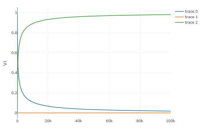
A delay differential equation is an ODE which allows the use of
previous values. In this case, the function needs to be a JIT compiled
Julia function. It looks just like the ODE, except in this case there is
a function h(p,t) which allows you to interpolate and grab
previous values.
We must provide a history function h(p,t) that gives
values for u before t0. Here we assume that
the solution was constant before the initial time point. Additionally,
we pass constant_lags = c(20.0) to tell the solver that
only constant-time lags were used and what the lag length was. This
helps improve the solver accuracy by accurately stepping at the points
of discontinuity. Together this is:
f <- JuliaCall::julia_eval("function f(du, u, h, p, t)
  du[1] = 1.1/(1 + sqrt(10)*(h(p, t-20)[1])^(5/4)) - 10*u[1]/(1 + 40*u[2])
  du[2] = 100*u[1]/(1 + 40*u[2]) - 2.43*u[2]
end")
h <- JuliaCall::julia_eval("function h(p, t)
  [1.05767027/3, 1.030713491/3]
end")
u0 <- c(1.05767027/3, 1.030713491/3)
tspan <- c(0.0, 100.0)
constant_lags <- c(20.0)
JuliaCall::julia_assign("u0", u0)
JuliaCall::julia_assign("tspan", tspan)
JuliaCall::julia_assign("constant_lags", tspan)
prob <- JuliaCall::julia_eval("DDEProblem(f, u0, h, tspan, constant_lags = constant_lags)")
sol <- de$solve(prob,de$MethodOfSteps(de$Tsit5()))
udf <- as.data.frame(t(sapply(sol$u,identity)))
plotly::plot_ly(udf, x = sol$t, y = ~V1, type = 'scatter', mode = 'lines') |> plotly::add_trace(y = ~V2)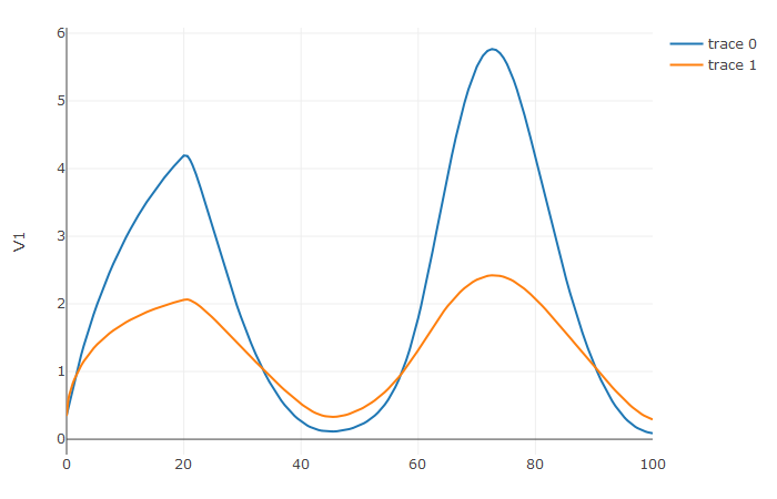
Notice that the solver accurately is able to simulate the kink
(discontinuity) at t=20 due to the discontinuity of the
derivative at the initial time point! This is why declaring
discontinuities can enhance the solver accuracy.
In many cases one is interested in solving the same ODE many times over many different initial conditions and parameters. In diffeqr parlance this is called an ensemble solve. diffeqr inherits the parallelism tools of the SciML ecosystem that are used for things like automated equation discovery and acceleration. Here we will demonstrate using these parallel tools to accelerate the solving of an ensemble.
First, let’s define the JIT-accelerated Lorenz equation like before:
de <- diffeqr::diffeq_setup()
lorenz <- function (u,p,t){
  du1 = p[1]*(u[2]-u[1])
  du2 = u[1]*(p[2]-u[3]) - u[2]
  du3 = u[1]*u[2] - p[3]*u[3]
  c(du1,du2,du3)
}
u0 <- c(1.0,1.0,1.0)
tspan <- c(0.0,100.0)
p <- c(10.0,28.0,8/3)
prob <- de$ODEProblem(lorenz,u0,tspan,p)
fastprob <- diffeqr::jitoptimize_ode(de,prob)
Now we use the EnsembleProblem as defined on the ensemble
parallelism page of the documentation: Let’s build an ensemble by
utilizing uniform random numbers to randomize the initial conditions and
parameters:
prob_func <- function (prob,i,rep){
  de$remake(prob,u0=runif(3)*u0,p=runif(3)*p)
}
ensembleprob = de$EnsembleProblem(fastprob, prob_func = prob_func, safetycopy=FALSE)
Now we solve the ensemble in serial:
sol = de$solve(ensembleprob,de$Tsit5(),de$EnsembleSerial(),trajectories=10000,saveat=0.01)To add GPUs to the mix, we need to bring in DiffEqGPU. The
diffeqr::diffeqgpu_setup() helper function will install
CUDA for you and bring all of the bindings into the returned object:
degpu <- diffeqr::diffeqgpu_setup("CUDA")diffeqr::diffeqgpu_setup can take awhile to run the first
time as it installs the drivers!Now we simply use EnsembleGPUKernel(degpu$CUDABackend())
with a GPU-specialized ODE solver GPUTsit5() to solve
10,000 ODEs on the GPU in parallel:
sol <- de$solve(ensembleprob,degpu$GPUTsit5(),degpu$EnsembleGPUKernel(degpu$CUDABackend()),trajectories=10000,saveat=0.01)For the full list of choices for specialized GPU solvers, see the DiffEqGPU.jl documentation.
Note that EnsembleGPUArray can be used as well,
like:
sol <- de$solve(ensembleprob,de$Tsit5(),degpu$EnsembleGPUArray(degpu$CUDABackend()),trajectories=10000,saveat=0.01)though we highly recommend the EnsembleGPUKernel methods
for more speed. Given the way the JIT compilation performed will also
ensure that the faster kernel generation methods work,
EnsembleGPUKernel is almost certainly the better choice in
most applications.
To see how much of an effect the parallelism has, let’s test this against R’s deSolve package. This is exactly the same problem as the documentation example for deSolve, so let’s copy that verbatim and then add a function to do the ensemble generation:
library(deSolve)
Lorenz <- function(t, state, parameters) {
  with(as.list(c(state, parameters)), {
    dX <-  a * X + Y * Z
    dY <-  b * (Y - Z)
    dZ <- -X * Y + c * Y - Z
    list(c(dX, dY, dZ))
  })
}

parameters <- c(a = -8/3, b = -10, c = 28)
state      <- c(X = 1, Y = 1, Z = 1)
times      <- seq(0, 100, by = 0.01)
out <- ode(y = state, times = times, func = Lorenz, parms = parameters)

lorenz_solve <- function (i){
  state      <- c(X = runif(1), Y = runif(1), Z = runif(1))
  parameters <- c(a = -8/3 * runif(1), b = -10 * runif(1), c = 28 * runif(1))
  out <- ode(y = state, times = times, func = Lorenz, parms = parameters)
}
Using lapply to generate the ensemble we get:
> system.time({ lapply(1:1000,lorenz_solve) })
   user  system elapsed
 225.81    0.46  226.63
Now let’s see how the JIT-accelerated serial Julia version stacks up against that:
> system.time({ de$solve(ensembleprob,de$Tsit5(),de$EnsembleSerial(),trajectories=1000,saveat=0.01) })
   user  system elapsed
   2.75    0.30    3.08
Julia is already about 73x faster than the pure R solvers here! Now let’s add GPU-acceleration to the mix:
> system.time({ de$solve(ensembleprob,degpu$GPUTsit5(),degpu$EnsembleGPUKernel(degpu$CUDABackend()),trajectories=1000,saveat=0.01) })
   user  system elapsed
   0.11    0.00    0.12
Already 26x times faster! But the GPU acceleration is made for massively parallel problems, so let’s up the trajectories a bit. We will not use more trajectories from R because that would take too much computing power, so let’s see what happens to the Julia serial and GPU at 10,000 trajectories:
> system.time({ de$solve(ensembleprob,de$Tsit5(),de$EnsembleSerial(),trajectories=10000,saveat=0.01) })
   user  system elapsed
  35.02    4.19   39.25
> system.time({ de$solve(ensembleprob,degpu$GPUTsit5(),degpu$EnsembleGPUKernel(degpu$CUDABackend()),trajectories=10000,saveat=0.01) })
user system elapsed
1.22 0.23 1.50 To compare this to the pure Julia code:
using OrdinaryDiffEq, DiffEqGPU, CUDA, StaticArrays
function lorenz(u, p, t)
    σ = p[1]
    ρ = p[2]
    β = p[3]
    du1 = σ * (u[2] - u[1])
    du2 = u[1] * (ρ - u[3]) - u[2]
    du3 = u[1] * u[2] - β * u[3]
    return SVector{3}(du1, du2, du3)
end

u0 = SA[1.0f0; 0.0f0; 0.0f0]
tspan = (0.0f0, 10.0f0)
p = SA[10.0f0, 28.0f0, 8 / 3.0f0]
prob = ODEProblem{false}(lorenz, u0, tspan, p)
prob_func = (prob, i, repeat) -> remake(prob, p = (@SVector rand(Float32, 3)) .* p)
monteprob = EnsembleProblem(prob, prob_func = prob_func, safetycopy = false)
@time sol = solve(monteprob, GPUTsit5(), EnsembleGPUKernel(CUDA.CUDABackend()),
    trajectories = 10_000,
    saveat = 1.0f0);

# 0.015064 seconds (257.68 k allocations: 13.132 MiB)
which is about two orders of magnitude faster for computing 10,000
trajectories, note that the major factors are that we cannot define
32-bit floating point values from R and the prob_func for
generating the initial conditions and parameters is a major bottleneck
since this function is written in R.
To see how this scales in Julia, let’s take it to insane heights. First, let’s reduce the amount we’re saving:
@time sol = solve(monteprob,GPUTsit5(),EnsembleGPUKernel(CUDA.CUDABackend()),trajectories=10_000,saveat=1.0f0)
0.015040 seconds (257.64 k allocations: 13.130 MiB)
This highlights that controlling memory pressure is key with GPU usage: you will get much better performance when requiring less saved points on the GPU.
@time sol = solve(monteprob,GPUTsit5(),EnsembleGPUKernel(CUDA.CUDABackend()),trajectories=100_000,saveat=1.0f0)
# 0.150901 seconds (2.60 M allocations: 131.576 MiB)
compared to serial:
@time sol = solve(monteprob,Tsit5(),EnsembleSerial(),trajectories=100_000,saveat=1.0f0)
# 22.136743 seconds (16.40 M allocations: 1.628 GiB, 42.98% gc time)
And now we start to see that scaling power! Let’s solve 1 million trajectories:
@time sol = solve(monteprob,GPUTsit5(),EnsembleGPUKernel(CUDA.CUDABackend()),trajectories=1_000_000,saveat=1.0f0)
# 1.031295 seconds (3.40 M allocations: 241.075 MiB)
For reference, let’s look at deSolve with the change to only save that much:
times      <- seq(0, 100, by = 1.0)
lorenz_solve <- function (i){
  state      <- c(X = runif(1), Y = runif(1), Z = runif(1))
  parameters <- c(a = -8/3 * runif(1), b = -10 * runif(1), c = 28 * runif(1))
  out <- ode(y = state, times = times, func = Lorenz, parms = parameters)
}

system.time({ lapply(1:1000,lorenz_solve) })
user system elapsed
49.69 3.36 53.42 The GPU version is solving 1000x as many trajectories, 50x as fast! So conclusion, if you need the most speed, you may want to move to the Julia version to get the most out of your GPU due to Float32’s, and when using GPUs make sure it’s a problem with a relatively average or low memory pressure, and these methods will give orders of magnitude acceleration compared to what you might be used to.