![]()
Read the methods paper here
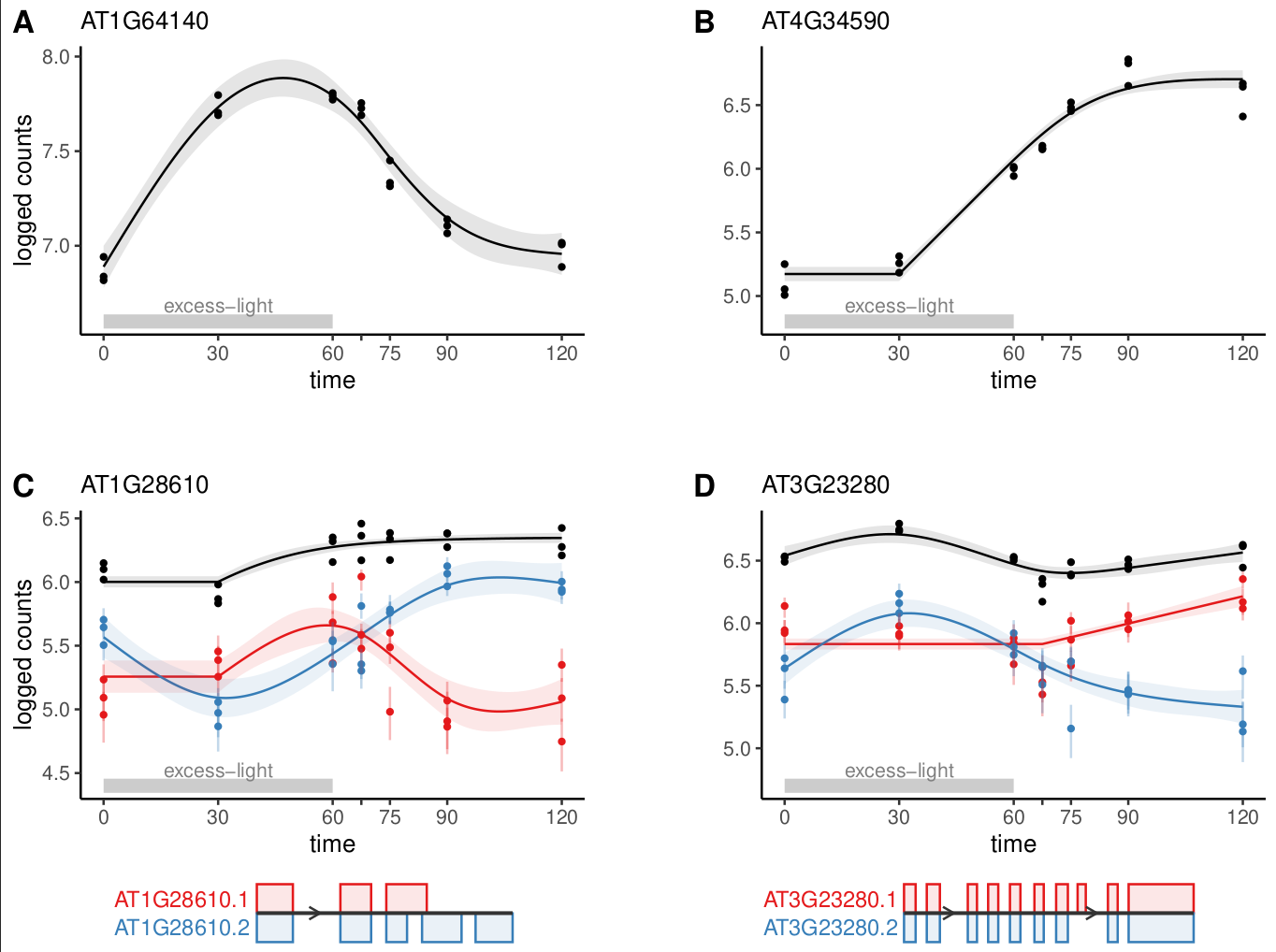
Application of cpam to RNA-seq time series of Arabidopsis plants treated with excess-light.
Our new package cpam provides a comprehensive framework for analysing time series omics data. The method uses modern statistical approaches while remaining user-friendly, through sensible defaults and an interactive interface. Researchers can directly address key questions in time series analysis—when changes occur, what patterns they follow, and how responses are related. While we have focused on transcriptomics, the framework is applicable to other high-dimensional time series measurements.
If you encounter issues or have suggestions for improvements, please open an issue. We welcome questions and discussion about using cpam for your research through Discussions. Our goal is to work with users to make cpam a robust and valuable tool for time series omics analysis. We can also be contacted via the email addresses listed in our paper here.
The package is available on CRAN and can be installed using the following command:
install.packages("cpam")For the development version, you can install it from GitHub using the
remotes package:
remotes::install_github("l-a-yates/cpam")library(cpam)In this Arabidopsis thaliana time series example, we used the software kallisto to generate counts from RNA-seq data. To load the counts, we provide the file path for each kallisto output file (alternatively you can provide the counts directly as count matrix, or use other quantification software)
# load example data
load(system.file("extdata", "exp_design_path.rda", package = "cpam"))
head(exp_design_path)
#>   sample time                                path condition
#> 1 JHSS01    0 output/kallisto/JHSS01/abundance.h5 treatment
#> 2 JHSS02    0 output/kallisto/JHSS02/abundance.h5 treatment
#> 3 JHSS03    0 output/kallisto/JHSS03/abundance.h5 treatment
#> 4 JHSS04    0 output/kallisto/JHSS04/abundance.h5 treatment
#> 5 JHSS05    0 output/kallisto/JHSS05/abundance.h5 treatment
#> 6 JHSS06 5 output/kallisto/JHSS06/abundance.h5 treatmentN.B. This is not needed if your counts are aggregated at the gene level, but transcript-level analysis with aggregation of \(p\)-values to the gene level is recommended. E.g., for Arabidopsis thaliana:
# load example data
load(system.file("extdata", "t2g_arabidopsis.rda", package = "cpam"))

head(t2g_arabidopsis)
#>     target_id   gene_id
#> 1 AT1G01010.1 AT1G01010
#> 2 AT1G01020.2 AT1G01020
#> 3 AT1G01020.6 AT1G01020
#> 4 AT1G01020.1 AT1G01020
#> 5 AT1G01020.4 AT1G01020
#> 6 AT1G01020.5 AT1G01020 cpo <- prepare_cpam(exp_design = exp_design_path,
count_matrix = NULL,
t2g = t2g_arabidopsis,
model = "case-only",
import_type = "kallisto",
num_cores = 5)
cpo <- compute_p_values(cpo)
cpo <- estimate_changepoint(cpo)
cpo <- select_shape(cpo) Load the shiny app for an interactive visualisation of the results:
visualise(cpo) # not shown in vignetteOr plot one gene at a time:
plot_cpam(cpo, gene_id = "AT3G23280")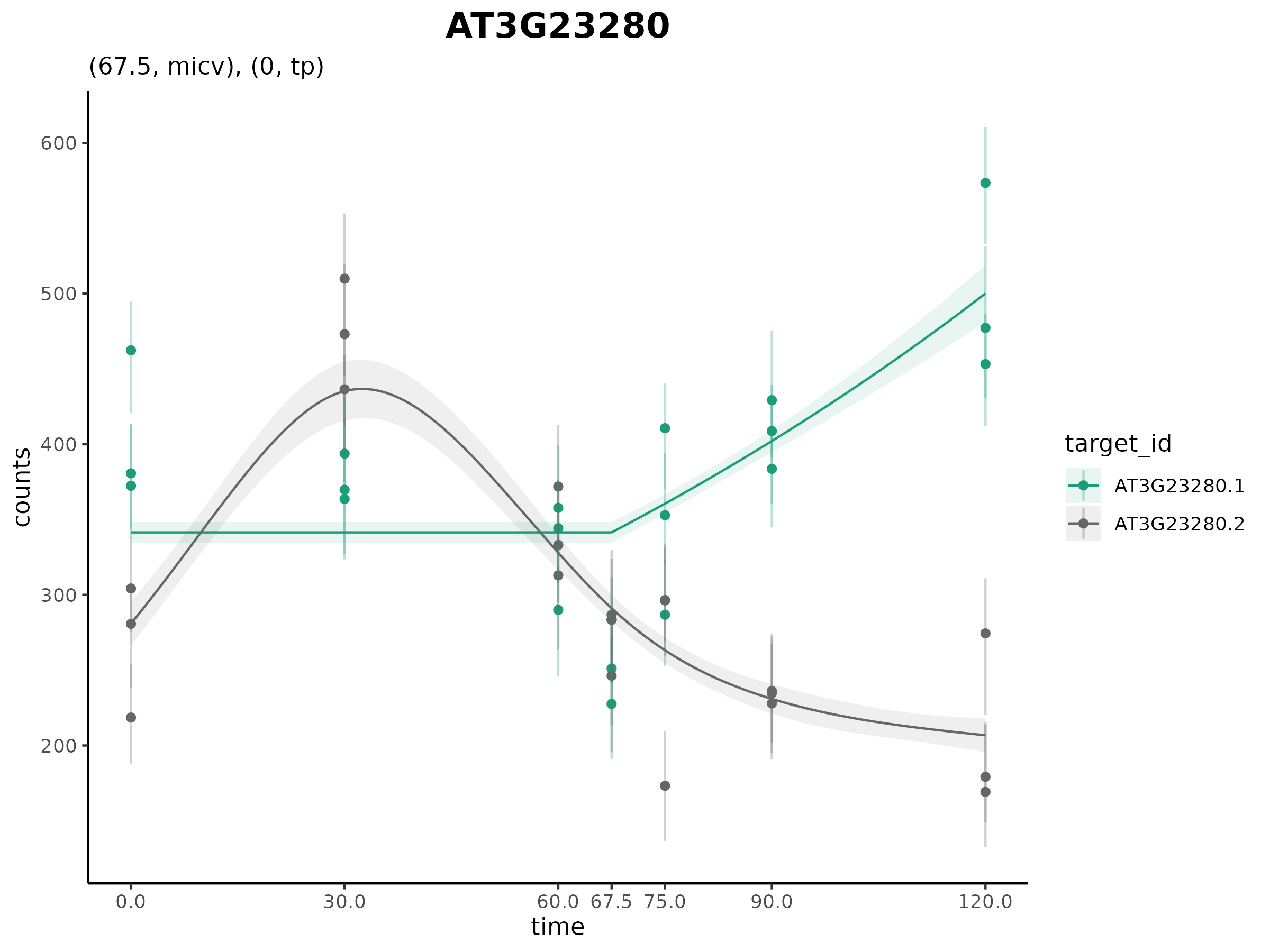
Isoform 1 (AT3G23280.1) has a changepoint at 67.5 min and has a
monotonic increasing concave (micv) shape. Isoform 2 (AT3G23280.2) has
no changepoint and has an unconstrained thin-plate (tp) shape.
We can generate a results table which has \(p\)-values, shapes, log-fold changes and counts with many optimal filters (see tutorials):
  results(cpo)
#> # A tibble: 15,279 × 25
#>    target_id   gene_id     p    cp shape lfc.0 lfc.5 lfc.10 lfc.20 lfc.30 lfc.45
#>    <chr>       <chr>   <dbl> <dbl> <chr> <dbl> <dbl>  <dbl>  <dbl>  <dbl>  <dbl>
#>  1 AT1G01910.1 AT1G01…     0     0 micv      0 1.01   1.70   2.38   2.60   2.73
#>  2 AT1G01910.2 AT1G01…     0    10 cv        0 0      0      0.553  0.775  0.790
#>  3 AT1G01910.5 AT1G01…     0    10 cx        0 0      0     -3.20  -4.57  -4.82
#>  4 AT1G02610.1 AT1G02…     0    45 mdcx      0 0      0      0      0      0
#>  5 AT1G02610.2 AT1G02…     0    10 cx        0 0      0     -0.645 -1.16  -1.71
#>  6 AT1G02610.3 AT1G02…     0    10 mdcx      0 0      0     -1.48  -2.11  -2.25
#>  7 AT1G04080.1 AT1G04…     0    10 cv        0 0      0      2.75   3.85   3.97
#>  8 AT1G04080.2 AT1G04…     0    45 micv      0 0      0      0      0      0
#>  9 AT1G04080.3 AT1G04…     0     0 micv      0 0.268  0.445  0.603  0.638  0.656
#> 10 AT1G04080.5 AT1G04…     0    10 cx        0 0      0     -2.17  -3.04  -3.10
#> # ℹ 15,269 more rows
#> # ℹ 14 more variables: lfc.60 <dbl>, lfc.90 <dbl>, lfc.180 <dbl>,
#> #   lfc.240 <dbl>, counts.0 <dbl>, counts.5 <dbl>, counts.10 <dbl>,
#> #   counts.20 <dbl>, counts.30 <dbl>, counts.45 <dbl>, counts.60 <dbl>,
#> # counts.90 <dbl>, counts.180 <dbl>, counts.240 <dbl>For a quick-to-run introductory example, we have provided a small simulated data set as part of the package.
The following two tutorials use real-world data to demonstrate the capabilities of the cpam package. In addition, they provide code to reproduce the results for the case studies presented in the manuscript accompanying the cpam package.
This work was supported by the Australian Research Council, Centre of Excellence for Plant Success in Nature and Agriculture (CE200100015).
![]()