![]()
![]()
The cmcR package provides an open-source implementation of the Congruent Matching Cells method for cartridge case identification as proposed by Song (2013) as well as the “High CMC” method proposed by Tong et al. (2015).
Install the development version from GitHub with:
# install.packages("devtools")
devtools::install_github("jzemmels/cmcR")
Cartridge case scan data can be accessed at the NIST Ballisitics Toolmark Research Database
We will illustrate the package’s functionality here. Please refer to the package vignettes available under the “Articles” tab of the package website for more information.
library(cmcR)
library(magrittr)
library(dplyr)
library(ggplot2)
library(x3ptools)
Consider the known match cartridge case pair Fadul 1-1 and Fadul 1-2.
The read_x3p function from the x3ptools package can read
scans from the NBTRD given the
appropriate address. The two scans are read below and visualized using
the x3pListPlot
function.
fadul1.1_id <- "DownloadMeasurement/2d9cc51f-6f66-40a0-973a-a9292dbee36d"
# Same source comparison
fadul1.2_id <- "DownloadMeasurement/cb296c98-39f5-46eb-abff-320a2f5568e8"

# Code to download breech face impressions:
nbtrd_url <- "https://tsapps.nist.gov/NRBTD/Studies/CartridgeMeasurement/"

fadul1.1_raw <- x3p_read(paste0(nbtrd_url,fadul1.1_id)) %>%
  x3ptools::x3p_scale_unit(scale_by = 1e6)
fadul1.2_raw <- x3p_read(paste0(nbtrd_url,fadul1.2_id)) %>%
  x3ptools::x3p_scale_unit(scale_by = 1e6)

x3pListPlot(list("Fadul 1-1" = fadul1.1_raw,
                 "Fadul 1-2" = fadul1.2_raw),
            type = "faceted")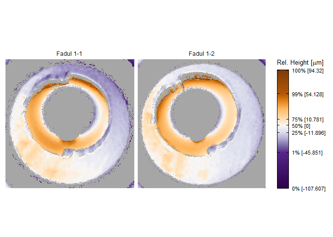
To perform a proper comparison of these two cartridge cases, we need
to remove regions that do not come into uniform or consistent contact
with the breech face of the firearm. These include the small clusters of
pixels in the corners of the two scans from the microscope staging area,
and the plateaued region of points around the firing pin impression hole
near the center of the scan. A variety of processing procedures are
implemented in the cmcR package. Functions of the form
preProcess_* perform the preprocessing procedures. See the
funtion
reference of the cmcR package for more information regarding these
procedures. As is commonly done when comparing cartridge cases, we
downsample each scan (by a factor of 4, selecting every other
row/column) using the sample_x3p function.
fadul1.1_processed <- fadul1.1_raw %>%
  preProcess_crop(region = "exterior",offset = -30) %>%
  preProcess_crop(region = "interior",offset = 200) %>%
  preProcess_removeTrend(statistic = "quantile",
                         tau = .5,
                         method = "fn") %>%
  preProcess_gaussFilter() %>%
  x3ptools::x3p_sample()

fadul1.2_processed <- fadul1.2_raw %>%
  preProcess_crop(region = "exterior",offset = -30) %>%
  preProcess_crop(region = "interior",offset = 200) %>%
  preProcess_removeTrend(statistic = "quantile",
                         tau = .5,
                         method = "fn") %>%
  preProcess_gaussFilter() %>%
  x3ptools::x3p_sample()

x3pListPlot(list("Processed Fadul 1-1" = fadul1.1_processed,
                 "Processed Fadul1-2" = fadul1.2_processed),
            type = "faceted")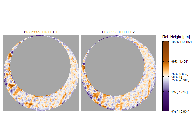
Functions of the form comparison_* perform the steps of
the cell-based comparison procedure. The data generated from the
cell-based comparison procedure are kept in a tibble where one
row represents a single cell/region pairing.
The comparison_cellDivision function divides a scan up
into a grid of cells. The cellIndex column represents the
row,col location in the original scan each cell inhabits.
Each cell is stored as an .x3p object in the
cellHeightValues column. The benefit of using a
tibble structure is that processes such as removing rows
can be accomplished using simple dplyr commands such as
filter.
cellTibble <- fadul1.1_processed %>%
  comparison_cellDivision(numCells = c(8,8))

cellTibble
#> # A tibble: 64 x 2
#>    cellIndex cellHeightValues
#>    <chr>     <named list>
#>  1 1, 1      <x3p>
#>  2 1, 2      <x3p>
#>  3 1, 3      <x3p>
#>  4 1, 4      <x3p>
#>  5 1, 5      <x3p>
#>  6 1, 6      <x3p>
#>  7 1, 7      <x3p>
#>  8 1, 8      <x3p>
#>  9 2, 1      <x3p>
#> 10 2, 2      <x3p>
#> # ... with 54 more rows
The comparison_getTargetRegions function extracts a
region from a target scan (in this case Fadul 1-2) to be paired with
each cell in the reference scan.
cellTibble <- cellTibble %>%
  mutate(regionHeightValues = comparison_getTargetRegions(cellHeightValues = cellHeightValues,
                                                          target = fadul1.2_processed))

cellTibble
#> # A tibble: 64 x 3
#>    cellIndex cellHeightValues regionHeightValues
#>    <chr>     <named list>     <named list>
#>  1 1, 1      <x3p>            <x3p>
#>  2 1, 2      <x3p>            <x3p>
#>  3 1, 3      <x3p>            <x3p>
#>  4 1, 4      <x3p>            <x3p>
#>  5 1, 5      <x3p>            <x3p>
#>  6 1, 6      <x3p>            <x3p>
#>  7 1, 7      <x3p>            <x3p>
#>  8 1, 8      <x3p>            <x3p>
#>  9 2, 1      <x3p>            <x3p>
#> 10 2, 2      <x3p>            <x3p>
#> # ... with 54 more rows
We want to exclude cells and regions that are mostly missing from the
scan. The comparison_calcPropMissing function calculates
the proportion of missing values in a surface matrix. The call below
excludes rows in which either the cell or region contain more that 85%
missing values.
cellTibble <- cellTibble %>%
  mutate(cellPropMissing = comparison_calcPropMissing(cellHeightValues),
         regionPropMissing = comparison_calcPropMissing(regionHeightValues)) %>%
  filter(cellPropMissing <= .85 & regionPropMissing <= .85)

cellTibble %>%
  select(cellIndex,cellPropMissing,regionPropMissing)
#> # A tibble: 24 x 3
#>    cellIndex cellPropMissing regionPropMissing
#>    <chr>               <dbl>             <dbl>
#>  1 1, 6               0.809              0.805
#>  2 2, 7               0.624              0.699
#>  3 2, 8               0.846              0.756
#>  4 3, 8               0.343              0.632
#>  5 4, 8               0.130              0.568
#>  6 5, 1               0.108              0.765
#>  7 5, 7               0.829              0.481
#>  8 5, 8               0.0522             0.508
#>  9 6, 1               0.314              0.689
#> 10 6, 2               0.340              0.602
#> # ... with 14 more rows
We can standardize the surface matrix height values by
centering/scaling by desired functions (e.g., mean and standard
deviation). Also, to apply frequency-domain techniques in comparing each
cell and region, the missing values in each scan need to be replaced.
These operations are performed in the
comparison_standardizeHeightValues and
comparison_replaceMissingValues functions.
Then, the comparison_fft_ccf function estimates the
translations required to align the cell and region using the Cross-Correlation
Theorem. The comparison_fft_ccf function returns a data
frame of 3 x, y, and fft_ccf
values: the estimated translation values at which the
CCF
value is attained between the cell and
region. The
tidyr::unnest function can unpack the data
frame into 3 separate columns, if desired.
cellTibble <- cellTibble  %>%
  mutate(cellHeightValues = comparison_standardizeHeights(cellHeightValues),
         regionHeightValues = comparison_standardizeHeights(regionHeightValues)) %>%
  mutate(cellHeightValues_replaced = comparison_replaceMissing(cellHeightValues),
         regionHeightValues_replaced = comparison_replaceMissing(regionHeightValues)) %>%
  mutate(fft_ccf_df = comparison_fft_ccf(cellHeightValues = cellHeightValues_replaced,
                                         regionHeightValues = regionHeightValues_replaced))

cellTibble %>%
  tidyr::unnest(cols = fft_ccf_df) %>%
  select(cellIndex,fft_ccf,x,y)
#> # A tibble: 24 x 4
#>    cellIndex fft_ccf     x     y
#>    <chr>       <dbl> <dbl> <dbl>
#>  1 1, 6        0.242    -6   -24
#>  2 2, 7        0.184    55    32
#>  3 2, 8        0.213    53    54
#>  4 3, 8        0.158   -22   -60
#>  5 4, 8        0.176    -2    13
#>  6 5, 1        0.211   -15   -47
#>  7 5, 7        0.117    21    16
#>  8 5, 8        0.166     8   -48
#>  9 6, 1        0.322   -56   -78
#> 10 6, 2        0.272     8   -46
#> # ... with 14 more rows
Because so many missing values need to be replaced, the CCF value calculated in the
fft_ccf column using frequency-domain techniques is not a
very good similarity score (doesn’t differentiate matches from
non-matches well). However, the x and y
estimated translations are good estimates of the “true” translation
values needed to align the cell and region. To calculate a more accurate
similarity score, we can use the pairwise-complete correlation in which
only pairs of non-missing pixels are considered in the correlation
calculation. To calculate this the
comparison_alignedTargetCell function takes the cell,
region, and CCF-based alignment information and returns a matrix of the
same dimension as the reference cell representing the sub-matrix of the
target region that the cell aligned to. We can then calculate the
pairwise-complete correlation as shown below.
cellTibble %>%
  dplyr::mutate(alignedTargetCell = comparison_alignedTargetCell(cellHeightValues = .data$cellHeightValues,
                                                                   regionHeightValues = .data$regionHeightValues,
                                                                   target = fadul1.2_processed,
                                                                   theta = 0,
                                                                   fft_ccf_df = .data$fft_ccf_df)) %>%
    dplyr::mutate(pairwiseCompCor = purrr::map2_dbl(.data$cellHeightValues,.data$alignedTargetCell,
                                             ~ cor(c(.x$surface.matrix),c(.y$surface.matrix),
                                                   use = "pairwise.complete.obs"))) %>%
    tidyr::unnest(.data$fft_ccf_df) %>%
  select(cellIndex,x,y,pairwiseCompCor)
#> # A tibble: 24 x 4
#>    cellIndex     x     y pairwiseCompCor
#>    <chr>     <dbl> <dbl>           <dbl>
#>  1 1, 6         -6   -24           0.558
#>  2 2, 7         55    32           0.377
#>  3 2, 8         53    54           0.751
#>  4 3, 8        -22   -60           0.373
#>  5 4, 8         -2    13           0.420
#>  6 5, 1        -15   -47           0.449
#>  7 5, 7         21    16           0.511
#>  8 5, 8          8   -48           0.355
#>  9 6, 1        -56   -78           0.590
#> 10 6, 2          8   -46           0.555
#> # ... with 14 more rows
Finally, this entire comparison procedure is to be repeated over a
number of rotations of the target scan. The entire cell-based comparison
procedure is wrapped in the comparison_allTogether
function. The resulting data frame below contains the features that are
used in the decision-rule procedure
kmComparisonFeatures <- purrr::map_dfr(seq(-30,30,by = 3),
                                       ~ comparison_allTogether(reference = fadul1.1_processed,
                                                                target = fadul1.2_processed,

                                                                theta = .,
                                                                returnX3Ps = TRUE))

kmComparisonFeatures %>%
  arrange(theta,cellIndex)
#> # A tibble: 506 x 11
#>    cellIndex     x     y fft_ccf pairwiseCompCor theta refMissingCount
#>    <chr>     <dbl> <dbl>   <dbl>           <dbl> <dbl>           <dbl>
#>  1 2, 7        -28   -54   0.203           0.399   -30            2970
#>  2 3, 1        -22    38   0.414           0.778   -30            2301
#>  3 3, 8        -17   -21   0.255           0.612   -30            1584
#>  4 4, 1        -11    35   0.287           0.756   -30            1467
#>  5 4, 8         -8   -25   0.230           0.656   -30             610
#>  6 5, 1         -1    35   0.300           0.677   -30             516
#>  7 5, 7          2    19   0.113           0.479   -30            3946
#>  8 5, 8          1   -22   0.227           0.599   -30             245
#>  9 6, 1          7    34   0.433           0.793   -30            1475
#> 10 6, 2         10    28   0.282           0.801   -30            1594
#> # ... with 496 more rows, and 4 more variables: targMissingCount <dbl>,
#> #   jointlyMissing <dbl>, cellHeightValues <named list>,
#> # alignedTargetCell <named list>The decision rules described in Song
(2013) and Tong
et al. (2015) are implemented via the decision_*
functions. We refer to the two decision rules as the original method of
Song
(2013) and the High CMC method, respectively. Considering the
kmComparisonFeatures data frame returned above, we can
interpret both of these decision rules as logic that separates
“aberrant” from “homogeneous” similarity features. The two decision
rules principally differ in how they define an homogeneity.
The original method of Song
(2013) considers only the similarity features at which the maximum
correlation is attained for each cell across all rotations considered.
Since there is ambiguity in exactly how the correlation is computed in
the original methods, we will consider the features at which
specifically the maximum pairwiseCompCor is attained
(instead of using the fft_ccf column).
kmComparisonFeatures %>%
  group_by(cellIndex) %>%
  top_n(n = 1,wt = pairwiseCompCor)
#> # A tibble: 26 x 11
#> # Groups:   cellIndex [26]
#>    cellIndex     x     y fft_ccf pairwiseCompCor theta refMissingCount
#>    <chr>     <dbl> <dbl>   <dbl>           <dbl> <dbl>           <dbl>
#>  1 7, 6         21    -1   0.147           0.471   -30             341
#>  2 4, 8         -7   -12   0.246           0.702   -27             610
#>  3 7, 4          7    10   0.215           0.721   -27            1908
#>  4 8, 5         10     6   0.247           0.603   -27             244
#>  5 2, 7        -14   -33   0.228           0.432   -24            2970
#>  6 3, 8         -7     5   0.277           0.699   -24            1584
#>  7 4, 1         -4    11   0.375           0.850   -24            1467
#>  8 5, 1         -4    11   0.363           0.852   -24             516
#>  9 6, 1         -3    11   0.437           0.832   -24            1475
#> 10 6, 2         -1    10   0.302           0.849   -24            1594
#> # ... with 16 more rows, and 4 more variables: targMissingCount <dbl>,
#> #   jointlyMissing <dbl>, cellHeightValues <named list>,
#> #   alignedTargetCell <named list>
The above set of features can be thought of as the x,
y, and theta “votes” that each cell most
strongly “believes” to be the correct alignment of the entire scan. If a
pair is truly matching, we would expect many of these votes to be
similar to each other; indicating that there is an approximate consensus
of the true alignment of the entire scan (at least, this is the
assumption made in Song
(2013)). In Song
(2013), the consensus is defined to be the median of the
x, y, and theta values in this
topVotesPerCell data frame. Cells that are deemed “close”
to these consensus values and that have a “large” correlation value are
declared Congruent Matching Cells (CMCs). Cells with x,
y, and theta values that are within
user-defined ,
, and
thresholds of the consensus
x, y, and theta values are
considered “close.” If these cells also have a correlation greater than
a user-defined threshold, then they are
considered CMCs. Note that these thresholds are chosen entirely by
experimentation in the CMC literature.
kmComparison_originalCMCs <- kmComparisonFeatures %>%
  mutate(originalMethodClassif = decision_CMC(cellIndex = cellIndex,
                                              x = x,
                                              y = y,
                                              theta = theta,
                                              corr = pairwiseCompCor,
                                              xThresh = 20,
                                              yThresh = 20,
                                              thetaThresh = 6,
                                              corrThresh = .5))

kmComparison_originalCMCs %>%
  filter(originalMethodClassif == "CMC")
#> # A tibble: 18 x 12
#>    cellIndex     x     y fft_ccf pairwiseCompCor theta refMissingCount
#>    <chr>     <dbl> <dbl>   <dbl>           <dbl> <dbl>           <dbl>
#>  1 4, 8         -7   -12   0.246           0.702   -27             610
#>  2 7, 4          7    10   0.215           0.721   -27            1908
#>  3 8, 5         10     6   0.247           0.603   -27             244
#>  4 3, 8         -7     5   0.277           0.699   -24            1584
#>  5 4, 1         -4    11   0.375           0.850   -24            1467
#>  6 5, 1         -4    11   0.363           0.852   -24             516
#>  7 6, 1         -3    11   0.437           0.832   -24            1475
#>  8 6, 2         -1    10   0.302           0.849   -24            1594
#>  9 6, 8         -4     7   0.324           0.787   -24            1475
#> 10 7, 1         -4     8   0.172           0.771   -24            4026
#> 11 7, 2         -2    10   0.253           0.768   -24             305
#> 12 7, 3         -1     7   0.199           0.736   -24             572
#> 13 7, 7         -3     3   0.366           0.829   -24             331
#> 14 8, 3         -1    12   0.279           0.747   -24            1447
#> 15 8, 4         -2     8   0.247           0.738   -24             235
#> 16 5, 8         -6    14   0.254           0.717   -21             245
#> 17 8, 6        -13    13   0.283           0.705   -21            1475
#> 18 3, 1          5    -9   0.516           0.855   -18            2301
#> # ... with 5 more variables: targMissingCount <dbl>, jointlyMissing <dbl>,
#> #   cellHeightValues <named list>, alignedTargetCell <named list>,
#> #   originalMethodClassif <chr>
Many have pointed out that there tends to be many cell/region pairs
that exhibit high correlation other than at the “true” rotation (theta)
value.
In particular, a cell/region pair may attain a very high correlation at
the “true” theta value, yet attain its maximum correlation at a theta
value far from the consensus theta value. The original method of Song
(2013) is quite sensitive to this behavior. The original method of
Song
(2013) only considers the “top” vote of each cell/region pairing, so
it is not sensitive to how that cell/region pairing behaves across
multiple rotations.
Tong
et al. (2015) propose a different decision rule procedure that
considers the behavior of cell/region pairings across multiple
rotations. This method would come to be called the High CMC method. The
procedure involves computing a “CMC-theta” distribution
where for each value of theta, the x and
y values are compared to consensus x and
y values (again, the median) and the correlation values to
a minimum threshold. A cell is considered a “CMC candidate” (our
language, not theirs) at a particular theta value if its
x and y values are within ,
thresholds of the consensus
x and
y values and the correlation is at least as larges as the
threshold. This is
similar to the original method of Song
(2013) except that it relaxes the requirement that the top
theta value be close to a consensus. Continuing with the
voting analogy, think of this as an approval voting
system where each cell is allowed to vote for multiple
theta values as long as the x and
y votes are deemed close to the theta-specific
x,y consensuses and the correlation values are
sufficiently high.
The CMC-theta distribution consists of the “CMC
candidates” at each value of theta. The assumption made in
Tong
et al. (2015) is that, for a truly matching cartridge case pair, a
large number of CMC candidates should be concentrated around true
theta alignment value. In their words, the
CMC-theta distribution should exhibit a “prominent peak”
close to the rotation at which the two cartridge cases actually align.
Such a prominent peak should not occur for a non-match cartridge case
pair.
The figure below shows an example of a CMC-theta
distribution between Fadul 1-1 and Fadul 1-2 constructed using the
decision_highCMC_cmcThetaDistrib function. We can clearly
see that a mode is attained around -24 degrees.
kmComparisonFeatures %>%
  mutate(cmcThetaDistribClassif = decision_highCMC_cmcThetaDistrib(cellIndex = cellIndex,
                                                                   x = x,
                                                                   y = y,
                                                                   theta = theta,
                                                                   corr = pairwiseCompCor,
                                                                   xThresh = 20,
                                                                   yThresh = 20,
                                                                   corrThresh = .5)) %>%
  filter(cmcThetaDistribClassif == "CMC Candidate") %>%
  ggplot(aes(x = theta)) +
  geom_bar(stat = "count",
           alpha = .7) +
  theme_bw() +
  ylab("CMC Candidate Count") +
  xlab(expression(theta))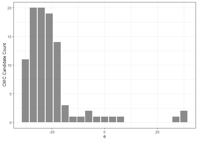
The next step of the High CMC method is to automatically determine if
a mode (i.e., a “prominent peak”) exists in a CMC-theta
distribution. If we find a mode, then there is evidence that a “true”
rotation exists to align the two cartridge cases implying the cartridge
cases must be matches (such is the logic employed in Tong
et al. (2015)). To automatically identify a mode, Tong
et al. (2015) propose determining the range of theta
values with “high” CMC candidate counts (if this range is small, then
there is likely a mode). They define a “high” CMC candidate count to be
where
is the maximum value attained in
the CMC-
theta distribution (17 in the plot shown above) and
is a user-defined constant (Tong
et al. (2015) use
). Any
theta value with
associated an associated CMC candidate count at least as large as have a “high” CMC
candidate count while any others have a “low” CMC candidate count.
The figure below shows the classification of theta
values into “High” and “Low” CMC candidate count groups using the
decision_highCMC_identifyHighCMCThetas function. The High
CMC count threshold is shown as a dashed line at CMCs.
kmComparisonFeatures %>%
  mutate(cmcThetaDistribClassif = decision_highCMC_cmcThetaDistrib(cellIndex = cellIndex,
                                                                   x = x,
                                                                   y = y,
                                                                   theta = theta,
                                                                   corr = pairwiseCompCor,
                                                                   xThresh = 20,
                                                                   yThresh = 20,
                                                                   corrThresh = .5)) %>%
  decision_highCMC_identifyHighCMCThetas(tau = 1) %>%
  filter(cmcThetaDistribClassif == "CMC Candidate") %>%
  ggplot() +
  geom_bar(aes(x = theta, fill = thetaCMCIdentif),
           stat = "count",
           alpha = .7) +
  geom_hline(aes(yintercept = max(cmcCandidateCount) - 1),
             linetype = "dashed") +
  scale_fill_manual(values = c("black","gray50")) +
  theme_bw() +
  ylab("CMC Candidate Count") +
  xlab(expression(theta))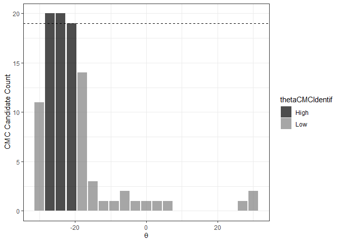
If the range of High CMC count theta values is less than
the user-defined threshold, then Tong
et al. (2015) classify all CMC candidates in the identified
theta mode as actual CMCs.
The decision_CMC function classifies CMCs based on this
High CMC criterion if a value for tau is given. Note that
it internally calls the decision_highCMC_cmcThetaDistrib
and decision_highCMC_identifyHighCMCThetas functions
(although they are exported as diagnostic tools). A cell may be counted
as a CMC for multiple theta values. In these cases, we will
only consider the alignment values at which the cell attained its
maximum CCF and was classified as a CMC. If the cartridge case pair
“fails” the High CMC criterion (i.e., the range of High CMC candidate
theta values is deemed too large), every cell will be
classified as “non-CMC (failed)” under the High CMC method. When it
comes to combining the CMCs from two comparison directions (cartridge
case A vs. B and B vs. A), we must treat a cell classified as a non-CMC
because the High CMC criterion failed differently from a cell classified
as a non-CMC for which the High CMC criterion passed.
kmComparison_highCMCs <- kmComparisonFeatures %>%
  mutate(highCMCClassif = decision_CMC(cellIndex = cellIndex,
                                       x = x,
                                       y = y,
                                       theta = theta,
                                       corr = pairwiseCompCor,
                                       xThresh = 20,
                                       yThresh = 20,
                                       thetaThresh = 6,
                                       corrThresh = .5,
                                       tau = 1))
#Example of cells classified as CMCs and non-CMCs
kmComparison_highCMCs %>%
  slice(21:35)
#> # A tibble: 15 x 12
#>    cellIndex     x     y fft_ccf pairwiseCompCor theta refMissingCount
#>    <chr>     <dbl> <dbl>   <dbl>           <dbl> <dbl>           <dbl>
#>  1 8, 3         21    24   0.295           0.719   -30            1447
#>  2 8, 4         69    20   0.228           0.481   -30             235
#>  3 8, 5         22     4   0.231           0.556   -30             244
#>  4 8, 6         23     2   0.204           0.565   -30            1475
#>  5 2, 7        -21   -43   0.218           0.421   -27            2970
#>  6 2, 8          3   -56   0.189           0.502   -27            3969
#>  7 3, 1        -14    27   0.443           0.808   -27            2301
#>  8 3, 8        -12    -8   0.269           0.664   -27            1584
#>  9 4, 1         -7    23   0.335           0.816   -27            1467
#> 10 4, 8         -7   -12   0.246           0.702   -27             610
#> 11 5, 1         -3    23   0.342           0.799   -27             516
#> 12 5, 7         53   -62   0.117           0.449   -27            3946
#> 13 5, 8         -2   -10   0.250           0.669   -27             245
#> 14 6, 1          2    22   0.437           0.814   -27            1475
#> 15 6, 2          5    19   0.294           0.827   -27            1594
#> # ... with 5 more variables: targMissingCount <dbl>, jointlyMissing <dbl>,
#> #   cellHeightValues <named list>, alignedTargetCell <named list>,
#> #   highCMCClassif <chr>
In summary: the decison_CMC function applies either the
decision rules of the original method of Song
(2013) or the High CMC method of Tong
et al. (2015), depending on whether the user specifies a value for
the High CMC threshold tau.
kmComparison_allCMCs <- kmComparisonFeatures %>%
  mutate(originalMethodClassif = decision_CMC(cellIndex = cellIndex,
                                              x = x,
                                              y = y,
                                              theta = theta,
                                              corr = pairwiseCompCor,
                                              xThresh = 20,
                                              thetaThresh = 6,
                                              corrThresh = .5),
         highCMCClassif = decision_CMC(cellIndex = cellIndex,
                                       x = x,
                                       y = y,
                                       theta = theta,
                                       corr = pairwiseCompCor,
                                       xThresh = 20,
                                       thetaThresh = 6,
                                       corrThresh = .5,
                                       tau = 1))

#Example of cells classified as CMC under 1 decision rule but not the other.
kmComparison_allCMCs %>%
  slice(21:35)
#> # A tibble: 15 x 13
#>    cellIndex     x     y fft_ccf pairwiseCompCor theta refMissingCount
#>    <chr>     <dbl> <dbl>   <dbl>           <dbl> <dbl>           <dbl>
#>  1 8, 3         21    24   0.295           0.719   -30            1447
#>  2 8, 4         69    20   0.228           0.481   -30             235
#>  3 8, 5         22     4   0.231           0.556   -30             244
#>  4 8, 6         23     2   0.204           0.565   -30            1475
#>  5 2, 7        -21   -43   0.218           0.421   -27            2970
#>  6 2, 8          3   -56   0.189           0.502   -27            3969
#>  7 3, 1        -14    27   0.443           0.808   -27            2301
#>  8 3, 8        -12    -8   0.269           0.664   -27            1584
#>  9 4, 1         -7    23   0.335           0.816   -27            1467
#> 10 4, 8         -7   -12   0.246           0.702   -27             610
#> 11 5, 1         -3    23   0.342           0.799   -27             516
#> 12 5, 7         53   -62   0.117           0.449   -27            3946
#> 13 5, 8         -2   -10   0.250           0.669   -27             245
#> 14 6, 1          2    22   0.437           0.814   -27            1475
#> 15 6, 2          5    19   0.294           0.827   -27            1594
#> # ... with 6 more variables: targMissingCount <dbl>, jointlyMissing <dbl>,
#> #   cellHeightValues <named list>, alignedTargetCell <named list>,
#> #   originalMethodClassif <chr>, highCMCClassif <chr>
The set of CMCs computed above are based on assuming Fadul 1-1 as the
reference scan and Fadul 1-2 as the target scan. Tong
et al. (2015) propose performing the cell-based comparison and
decision rule procedures with the roles reversed and combining the
results. They indicate that if the High CMC method fails to identify a
theta mode in the CMC-theta distribution, then
the minimum of the two CMC counts computed under the original method of
Song
(2013) should be used as the CMC count (although they don’t detail
how to proceed if a theta mode is identified in only one of
the two comparisons).
#Compare using Fadul 1-2 as reference and Fadul 1-1 as target
kmComparisonFeatures_rev <- purrr::map_dfr(seq(-30,30,by = 3),
                                           ~ comparison_allTogether(reference = fadul1.2_processed,
                                                                    target = fadul1.1_processed,
                                                                    theta = .))

kmComparison_allCMCs_rev <- kmComparisonFeatures_rev %>%
  mutate(originalMethodClassif = decision_CMC(cellIndex = cellIndex,
                                              x = x,
                                              y = y,
                                              theta = theta,
                                              corr = pairwiseCompCor,
                                              xThresh = 20,
                                              thetaThresh = 6,
                                              corrThresh = .5),
         highCMCClassif = decision_CMC(cellIndex = cellIndex,
                                       x = x,
                                       y = y,
                                       theta = theta,
                                       corr = pairwiseCompCor,
                                       xThresh = 20,
                                       thetaThresh = 6,
                                       corrThresh = .5,
                                       tau = 1))
The logic required to combine the results in
kmComparison_allCMCs and
kmComparison_allCMCs_rev can get a little complicated
(although entirely doable using dplyr and other
tidyverse functions). The user must decide precisely how
results from both directions are to be combined. For example, if one
direction fails the High CMC criterion yet the other passes, should we
treat this as if both directions failed? Will you only count
the CMCs in the direction that passed? We have found the best option to
be treating a failure in one direction as a failure in both directions –
such cartridge case pairs would then be assigned the minimum of the two
CMC counts determined under the original method of Song
(2013). The decision_combineDirections function
implements the logic to combine the two sets of results, assuming the
data frame contains columns named originalMethodClassif and
highCMCClassif (as defined above).
decision_combineDirections(kmComparison_allCMCs %>%
                             select(-c(cellHeightValues,alignedTargetCell)),
                           kmComparison_allCMCs_rev)
#> $originalMethodCMCs
#> $originalMethodCMCs[[1]]
#> # A tibble: 18 x 10
#>    cellIndex     x     y fft_ccf pairwiseCompCor theta refMissingCount
#>    <chr>     <dbl> <dbl>   <dbl>           <dbl> <dbl>           <dbl>
#>  1 4, 8         -7   -12   0.246           0.702   -27             610
#>  2 7, 4          7    10   0.215           0.721   -27            1908
#>  3 8, 5         10     6   0.247           0.603   -27             244
#>  4 3, 8         -7     5   0.277           0.699   -24            1584
#>  5 4, 1         -4    11   0.375           0.850   -24            1467
#>  6 5, 1         -4    11   0.363           0.852   -24             516
#>  7 6, 1         -3    11   0.437           0.832   -24            1475
#>  8 6, 2         -1    10   0.302           0.849   -24            1594
#>  9 6, 8         -4     7   0.324           0.787   -24            1475
#> 10 7, 1         -4     8   0.172           0.771   -24            4026
#> 11 7, 2         -2    10   0.253           0.768   -24             305
#> 12 7, 3         -1     7   0.199           0.736   -24             572
#> 13 7, 7         -3     3   0.366           0.829   -24             331
#> 14 8, 3         -1    12   0.279           0.747   -24            1447
#> 15 8, 4         -2     8   0.247           0.738   -24             235
#> 16 5, 8         -6    14   0.254           0.717   -21             245
#> 17 8, 6        -13    13   0.283           0.705   -21            1475
#> 18 3, 1          5    -9   0.516           0.855   -18            2301
#> # ... with 3 more variables: targMissingCount <dbl>, jointlyMissing <dbl>,
#> #   direction <chr>
#>
#> $originalMethodCMCs[[2]]
#> # A tibble: 17 x 10
#>    cellIndex     x     y fft_ccf pairwiseCompCor theta refMissingCount
#>    <chr>     <dbl> <dbl>   <dbl>           <dbl> <dbl>           <dbl>
#>  1 4, 1         -3    11   0.529           0.863    18            2850
#>  2 2, 7         -5   -16   0.262           0.637    21            1034
#>  3 6, 2          6    -2   0.217           0.770    21            2858
#>  4 6, 6          1   -14   0.269           0.796    21            3273
#>  5 7, 2          8    -3   0.463           0.827    21             306
#>  6 8, 5          9    -2   0.348           0.652    21             244
#>  7 3, 8          3    -5   0.294           0.677    24            1447
#>  8 4, 8          2    -6   0.369           0.783    24             235
#>  9 5, 1         -1   -13   0.361           0.837    24            1664
#> 10 5, 8          1    -8   0.387           0.811    24             244
#> 11 6, 1         -2   -11   0.348           0.831    24            1482
#> 12 6, 8          1    -3   0.489           0.885    24            1475
#> 13 7, 3         -1   -10   0.359           0.885    24             993
#> 14 7, 7         -3    -7   0.238           0.720    24             331
#> 15 8, 4         -4    -7   0.270           0.761    24             235
#> 16 7, 5        -11    -6   0.285           0.729    27            1213
#> 17 7, 6         -9     0   0.220           0.682    27              17
#> # ... with 3 more variables: targMissingCount <dbl>, jointlyMissing <dbl>,
#> #   direction <chr>
#>
#>
#> $highCMCs
#> # A tibble: 25 x 10
#>    cellIndex     x     y fft_ccf pairwiseCompCor theta refMissingCount
#>    <chr>     <dbl> <dbl>   <dbl>           <dbl> <dbl>           <dbl>
#>  1 7, 4          7    10   0.215           0.721   -27            1908
#>  2 3, 8         -7     5   0.277           0.699   -24            1584
#>  3 4, 1         -4    11   0.375           0.850   -24            1467
#>  4 5, 1         -4    11   0.363           0.852   -24             516
#>  5 6, 1         -3    11   0.437           0.832   -24            1475
#>  6 6, 2         -1    10   0.302           0.849   -24            1594
#>  7 6, 7         -4     4   0.167           0.592   -24             990
#>  8 7, 1         -4     8   0.172           0.771   -24            4026
#>  9 7, 7         -3     3   0.366           0.829   -24             331
#> 10 8, 3         -1    12   0.279           0.747   -24            1447
#> # ... with 15 more rows, and 3 more variables: targMissingCount <dbl>,
#> #   jointlyMissing <dbl>, direction <chr>
The final step is to decide whether the number of CMCs computed under your preferred method is large enough to declare the cartridge case a match. Song (2013) originally proposed using a CMC count equal to 6 as the decision boundary (i.e., classify “match” if CMC count is greater than or equal to 6). This has been shown to not generalize to other proposed methods and data sets (see, e.g., Chen et al. (2017)). A more principled approach to choosing the CMC count has not yet been described.
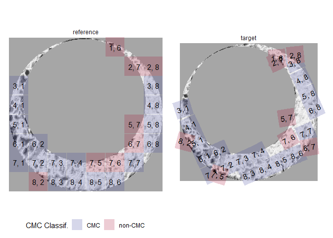
Finally, we can visualize the regions of the scan identified as CMCs.
cmcPlot(reference = fadul1.1_processed,
                    target  = fadul1.2_processed,
                    cmcClassifs = kmComparisonFeatures %>%
  mutate(originalMethodClassif = decision_CMC(cellIndex = cellIndex,
                                              x = x,
                                              y = y,
                                              theta = theta,
                                              corr = pairwiseCompCor,
                                              xThresh = 20,
                                              thetaThresh = 6,
                                              corrThresh = .5)) %>%
    group_by(cellIndex) %>%
    filter(pairwiseCompCor == max(pairwiseCompCor)),
                    cmcCol = "originalMethodClassif")