The goal of clustlearn is to provide a set of functions to perform clustering analysis along with comprehensive explanations of the algorithms, their pros and cons, and their applications.
You can install the released version of clustlearn from CRAN with:
install.packages("clustlearn")You can install the development version of clustlearn from GitHub with:
devtools::install_github("Ediu3095/clustlearn")This is a basic example which shows you how to cluster a dataset:
# # Load the clustlearn package
# library(clustlearn)
# Perform the clustering (the clustlearn:: prefix is not necessary)
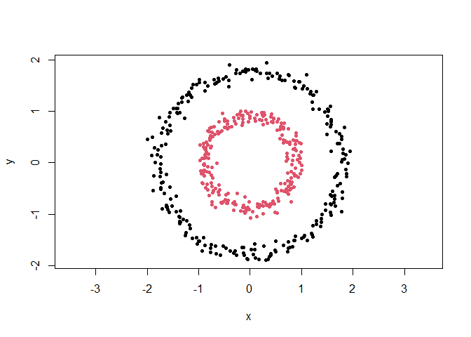
cl <- clustlearn::dbscan(clustlearn::db1, 0.3)
# Plot the results
out <- cl$cluster == 0
plot(clustlearn::db1[!out, ], col = cl$cluster[!out], pch = 20, asp = 1)
points(clustlearn::db1[out, ], col = max(cl$cluster) + 1, pch = 4, lwd = 2)
This is yet another basic example which shows you how to see the step-by-step procedure of the clustering algorithm:
# # Load the clustlearn package
# library(clustlearn)
# Perform the clustering (the clustlearn:: prefix is not necessary)
# The details argument is set to TRUE to see the step-by-step procedure
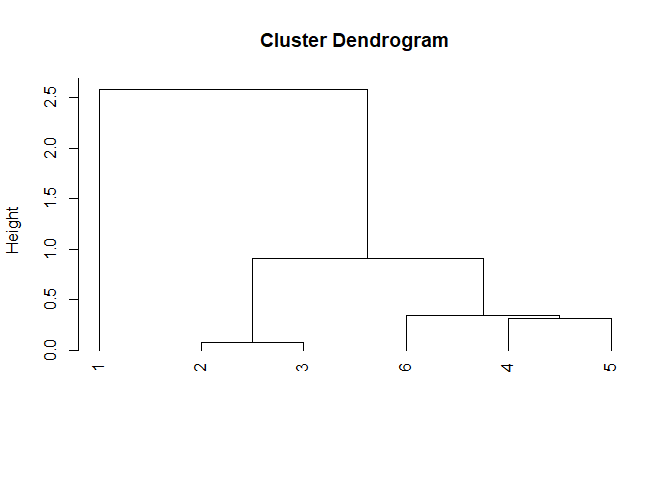
cl <- clustlearn::agglomerative_clustering(
clustlearn::db5[1:6, ],
'single',
details = TRUE,
waiting = FALSE
)## ________________________________________________________________________________
## EXPLANATION:
##
## The Agglomerative Hierarchical Clustering algorithm defines a clustering hierarc
## hy for a dataset following a `n` step process, which repeats until a single clus
## ter remains:
##
## 1. Initially, each object is assigned to its own cluster. The matrix of dist
## ances between clusters is computed.
## 2. The two clusters with closest proximity will be joined together and the p
## roximity matrix updated. This is done according to the specified proximity.
## This step is repeated until a single cluster remains.
##
## The definitions of proximity considered by this function are:
##
## 1. `single`. Defines the proximity between two clusters as the distance betw
## een the closest objects among the two clusters. It produces clusters where e
## ach object is closest to at least one other object in the same cluster. It i
## s known as SLINK, single-link or minimum-link.
## 2. `complete`. Defines the proximity between two clusters as the distance be
## tween the furthest objects among the two clusters. It is known as CLINK, com
## plete-link or maximum-link.
## 3. `average`. Defines the proximity between two clusters as the average dist
## ance between every pair of objects, one from each cluster. It is also known
## as UPGMA or average-link.
##
## ________________________________________________________________________________
## STEP 1:
##
## Initially, each object is assigned to its own cluster. This leaves us with the f
## ollowing clusters:
## CLUSTER #-1 (size: 1)
## x y
## 1 -1.578117 -1.292868
## CLUSTER #-2 (size: 1)
## x y
## 2 0.7027994 1.193823
## CLUSTER #-3 (size: 1)
## x y
## 3 0.7854535 1.191428
## CLUSTER #-4 (size: 1)
## x y
## 4 0.6757613 -0.04002442
## CLUSTER #-5 (size: 1)
## x y
## 5 0.8484305 0.2230609
## CLUSTER #-6 (size: 1)
## x y
## 6 0.515489 0.3014147
##
## The matrix of distances between clusters is computed:
## Distances:
## -1 -2 -3 -4 -5
## -2 3.374
## -3 3.429 0.083
## -4 2.579 1.234 1.236
## -5 2.861 0.982 0.970 0.315
## -6 2.632 0.912 0.930 0.377 0.342
##
## ________________________________________________________________________________
## STEP 2:
##
## The two clusters with closest proximity are identified:
## Clusters:
## CLUSTER #-2 (size: 1)
## CLUSTER #-3 (size: 1)
## Proximity:
## [1] 0.08268877
##
## They are merged into a new cluster:
## CLUSTER #1 (size: 2) [CLUSTER #-2 + CLUSTER #-3]
##
## The proximity matrix is updated. To do so the rows/columns of the merged cluster
## s are removed, and the rows/columns of the new cluster are added:
## Distances:
## -1 -4 -5 -6
## -4 2.579
## -5 2.861 0.315
## -6 2.632 0.377 0.342
## 1 3.374 1.234 0.970 0.912
##
## ________________________________________________________________________________
## STEP 3:
##
## The two clusters with closest proximity are identified:
## Clusters:
## CLUSTER #-4 (size: 1)
## CLUSTER #-5 (size: 1)
## Proximity:
## [1] 0.3146881
##
## They are merged into a new cluster:
## CLUSTER #2 (size: 2) [CLUSTER #-4 + CLUSTER #-5]
##
## The proximity matrix is updated. To do so the rows/columns of the merged cluster
## s are removed, and the rows/columns of the new cluster are added:
## Distances:
## -1 -6 1
## -6 2.632
## 1 3.374 0.912
## 2 2.579 0.342 0.970
##
## ________________________________________________________________________________
## STEP 4:
##
## The two clusters with closest proximity are identified:
## Clusters:
## CLUSTER #-6 (size: 1)
## CLUSTER #2 (size: 2)
## Proximity:
## [1] 0.342037
##
## They are merged into a new cluster:
## CLUSTER #3 (size: 3) [CLUSTER #-6 + CLUSTER #2]
##
## The proximity matrix is updated. To do so the rows/columns of the merged cluster
## s are removed, and the rows/columns of the new cluster are added:
## Distances:
## -1 1
## 1 3.374
## 3 2.579 0.912
##
## ________________________________________________________________________________
## STEP 5:
##
## The two clusters with closest proximity are identified:
## Clusters:
## CLUSTER #1 (size: 2)
## CLUSTER #3 (size: 3)
## Proximity:
## [1] 0.9118542
##
## They are merged into a new cluster:
## CLUSTER #4 (size: 5) [CLUSTER #1 + CLUSTER #3]
##
## The proximity matrix is updated. To do so the rows/columns of the merged cluster
## s are removed, and the rows/columns of the new cluster are added:
## Distances:
## -1
## 4 2.579
##
## ________________________________________________________________________________
## STEP 6:
##
## The two clusters with closest proximity are identified:
## Clusters:
## CLUSTER #-1 (size: 1)
## CLUSTER #4 (size: 5)
## Proximity:
## [1] 2.578678
##
## They are merged into a new cluster:
## CLUSTER #5 (size: 6) [CLUSTER #-1 + CLUSTER #4]
##
## The proximity matrix is updated. To do so the rows/columns of the merged cluster
## s are removed, and the rows/columns of the new cluster are added:
## Distances:
## dist(0)
##
## ________________________________________________________________________________
## RESULTS:
##
## Since all clusters have been merged together, the final clustering hierarchy is:
## (Check the plot for the dendrogram representation of the hierarchy)
##
## ________________________________________________________________________________