
The centerline R package simplifies the extraction of
linear features from complex polygons, such as roads or rivers, by
computing their centerlines (or median-axis) based on skeletons. It uses
the super-fast geos
library in the background and have bindings for your favorite spatial
data library (sf, terra and geos).
# The easiest way to get centerline is to install it from CRAN:
install.packages("centerline")

# Or the development version from GitHub:
# install.packages("pak")
pak::pak("atsyplenkov/centerline")At the heart of this package is the cnt_skeleton
function, which efficiently computes the skeleton of closed 2D polygonal
geometries. The function uses geos::geos_simplify
by default to keep the most important nodes and reduce noise from the
beginning. However, it has option to densify the amount of points using
geos::geos_densify,
which can produce more smooth results. Otherwise, you can set the
parameter keep = 1 to work with the initial geometry.
library(sf)
library(centerline)

lake <-
  sf::st_read(
    system.file("extdata/example.gpkg", package = "centerline"),
    layer = "lake",
    quiet = TRUE
  )

# Original
lake_skeleton <-
  cnt_skeleton(lake, keep = 1)

# Simplified
lake_skeleton_s <-
  cnt_skeleton(lake, keep = 0.1)

# Densified
lake_skeleton_d <-
cnt_skeleton(lake, keep = 2)library(ggplot2)
skeletons <-
rbind(lake_skeleton, lake_skeleton_s, lake_skeleton_d)
skeletons$type <- factor(
c("Original", "Simplified", "Densified"),
levels = c("Original", "Simplified", "Densified")
)
skeletons_plot <-
ggplot() +
geom_sf(
data = lake,
fill = "#c8e8f1",
color = NA
) +
geom_sf(
data = skeletons,
lwd = 0.2,
alpha = 0.5,
color = "#263238"
) +
coord_sf(expand = FALSE, clip = "off") +
labs(caption = "cnt_skeleton() example") +
facet_wrap(~type) +
theme_void() +
theme(
plot.caption = element_text(family = "mono", size = 6),
plot.background = element_rect(fill = "white", color = NA),
strip.text = element_text(face = "bold", hjust = 0.25, size = 12),
plot.margin = margin(0.2, -0.5, 0.2, -0.5, unit = "lines"),
panel.spacing.x = unit(-2, "lines")
)
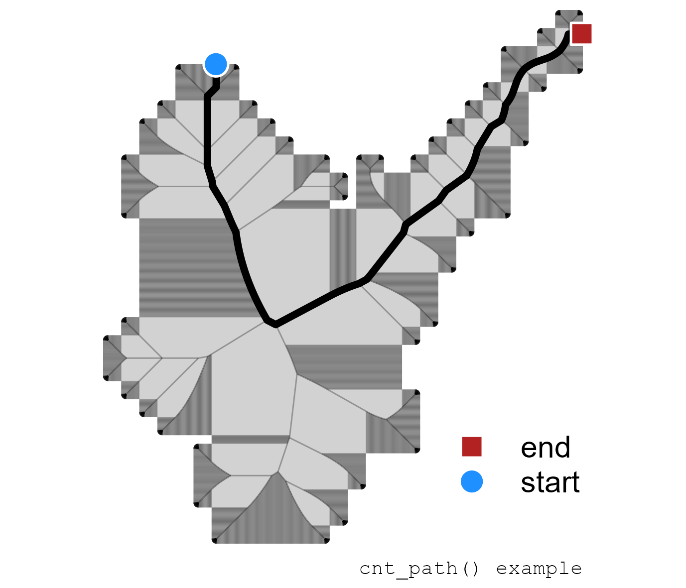
However, the above-generated lines are not exactly a centerline of a
polygon. One way to find the centerline of a closed polygon is to define
both start and end points with the
cnt_path() function. For example, in the case of
landslides, it could be the landslide initiation point and landslide
terminus.
# Load Polygon Of Interest (POI)
polygon <-
  sf::st_read(
    system.file(
      "extdata/example.gpkg",
      package = "centerline"
    ),
    layer = "polygon",
    quiet = TRUE
  )

# Load points data
points <-
  sf::st_read(
    system.file(
      "extdata/example.gpkg",
      package = "centerline"
    ),
    layer = "polygon_points",
    quiet = TRUE
  ) |>
  head(n = 2)
points$id <- seq_len(nrow(points))

# Find POI's skeleton
pol_skeleton <- cnt_skeleton(polygon, keep = 1.5)

# Connect points
# For original skeleton
pol_path <-
  cnt_path(
    skeleton = pol_skeleton,
    start_point = subset(points, points$type == "start"),
    end_point = subset(points, points$type == "end")
)path_plot <- ggplot() +
geom_sf(
data = polygon,
fill = "#d2d2d2",
color = NA
) +
geom_sf(
data = pol_path,
lwd = 1,
color = "black"
) +
geom_sf(
data = points,
aes(
shape = type,
fill = type
),
color = "white",
lwd = rel(1),
size = rel(3)
) +
scale_fill_manual(
name = "",
values = c(
"start" = "dodgerblue",
"end" = "firebrick"
)
) +
scale_shape_manual(
name = "",
values = c(
"start" = 21,
"end" = 22
)
) +
coord_sf(expand = FALSE, clip = "off") +
labs(caption = "cnt_path() example") +
theme_void() +
theme(
legend.position = "inside",
legend.position.inside = c(0.85, 0.2),
legend.key.spacing.y = unit(-0.5, "lines"),
plot.caption = element_text(family = "mono", size = 6),
plot.background = element_rect(fill = "white", color = NA),
strip.text = element_text(face = "bold", hjust = 0.25, size = 12),
plot.margin = margin(0.2, -0.5, 0.2, -0.5, unit = "lines"),
panel.spacing.x = unit(-2, "lines")
)
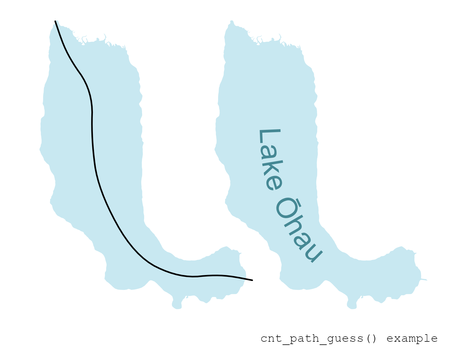
And what if we don’t know the starting and ending locations? What if
we just want to place our label accurately in the middle of our polygon?
In this case, one may find the cnt_path_guess function
useful. It returns the line connecting the most distant points, i.e.,
the polygon’s length. Such an approach is used in limnology for
measuring lake
lengths, for example.
lake_centerline <- cnt_path_guess(lake, keep = 1)You can plot polygon centerline with the geom_cnt_*
functions family:
library(ggplot2)

lakes <- rbind(lake, lake)
lakes$lc <- c("black", NA_character_)

centerline_plot <-
  ggplot() +
  geom_sf(
    data = lakes,
    fill = "#c8e8f1",
    color = NA
  ) +
  geom_cnt_text(
    data = lakes,
    aes(
      label = name,
      linecolor = lc
    ),
    keep = 1
  ) +
  facet_wrap(~lc) +
  labs(
    caption = "cnt_path_guess() and geom_cnt_text() examples"
  ) +
  theme_void() +
  theme(
    legend.position = "inside",
    legend.position.inside = c(0.85, 0.2),
    legend.key.spacing.y = unit(-0.5, "lines"),
    plot.caption = element_text(family = "mono", size = 6),
    plot.background = element_rect(fill = "white", color = NA),
    strip.text = element_blank(),
    plot.margin = margin(0.2, -0.5, 0.2, -0.5, unit = "lines"),
    panel.spacing.x = unit(-2, "lines")
  )
centerline 📦
├── Closed geometries (e.g., lakes, landslides)
│   ├── When we do know starting and ending points (e.g., landslides) ✅
│   │   ├── centerline::cnt_skeleton ✅
│   │   └── centerline::cnt_path ✅
│   └── When we do NOT have points (e.g., lakes) ✅
│       ├── centerline::cnt_skeleton ✅
│       └── centerline::cnt_path_guess ✅
├── Linear objects (e.g., roads or rivers)  🔲
└── Collapse parallel lines to centerline 🔲cnt_skeleton(method = "straight") function of the current
package.