![]()
Cellpypes uses the popular piping operator %>% to
manually annotate cell types in single-cell RNA sequencing data. It can
be applied to UMI data (e.g. 10x Genomics).
Define gene rules interactively:
feat, select with rule,
visualize with plot_last or plot_classes and
get cell type labels with classify.Resolve detailed cell type subsets. Switch between cell type hierarchy levels in your analysis:
Install cellpypes with the following commands:
# install.packages("devtools")
devtools::install_github("FelixTheStudent/cellpypes")To cite cellpypes, download your favorite citation style from zenodo, type
citation("cellpypes") in R or simply use:
Frauhammer, Felix, & Anders, Simon. (2022). cellpypes: Cell Type Pipes for R (0.1.1). Zenodo. https://doi.org/10.5281/zenodo.6555728
cellpypes input has four slots:
raw: (sparse) matrix with genes in rows, cells in
columnstotalUMI: the colSums of obj$rawembed: two-dimensional embedding of the cells, provided
as data.frame or tibble with two columns and one row per cell.neighbors: index matrix with one row per cell and
k-nearest neighbor indices in columns. We recommend k=50, but generally
15<k<100 works well. Here are two ways to get the
neighbors index matrix:
find_knn(featureMatrix)$idx, where featureMatrix
could be principal components, latent variables or normalized genes
(features in rows, cells in columns).as(seurat@graphs[["RNA_nn"]], "dgCMatrix")>.1 to
extract the kNN graph computed on RNA. This also works with RNA_snn,
wknn/wsnn or any other available graph – check with
names(seurat@graphs).Examples for cellpypes input:
# Object from scratch:
obj <- list(
  raw = counts,              # raw UMI, cells in columns
  neighbors = knn_ids,       # neighbor indices, cells in rows, k columns
  embed = umap,              # 2D embedding, cells in rows
  totalUMI = library_sizes   # colSums of raw, one value per cell
)

# Object from Seurat:
obj <- list(
    raw      =SeuratObject::GetAssayData(seurat, "counts"),
    neighbors=as(seurat@graphs[["RNA_nn"]], "dgCMatrix")>.1, # sometims "wknn"
    embed    =FetchData(seurat, dimension_names),
    totalUMI = seurat$nCount_RNA
)

# Object from Seurat (experimental short-cut):
obj <- pype_from_seurat(seurat_object)Functions for manual classification:
feat: feature plot (UMAP colored by gene
expression)rule: add a cell type ruleplot_last: plot the most recent rule or classclassify: classify cells by evaluating cell type
rulesplot_classes: call and visualize
classifyFunctions for pseudobulking and differential gene expression (DE) analysis:
class_to_deseq2: Create DESeq2 object for a given cell
typepseudobulk: Form pseudobulks from single-cellspseudobulk_id: Generate unique IDs to identify
pseudobulksHere, we annotate the same PBMC data set as in the popular Seurat
tutorial, using the Seurat object seurat_object that
comes out of it.
library(cellpypes)
library(tidyverse) # provides piping operator %>%


pype <- seurat_object %>%
  pype_from_seurat %>%
  rule("B",           "MS4A1",   ">", 1)                    %>%
  rule("CD14+ Mono",  "CD14",    ">", 1)                    %>%
  rule("CD14+ Mono",  "LYZ",     ">", 20)                   %>%
  rule("FCGR3A+ Mono","MS4A7",   ">", 2)                    %>%
  rule("NK",          "GNLY",    ">", 75)                   %>%
  rule("DC",          "FCER1A",  ">", 1)                    %>%
  rule("Platelet",    "PPBP",    ">", 30)                   %>%
  rule("T",           "CD3E",    ">", 3.5)                  %>%
  rule("CD8+ T",      "CD8A",    ">", .8,  parent="T")      %>%
  rule("CD4+ T",      "CD4",     ">", .05, parent="T")      %>%
  rule("Naive CD4+",  "CCR7",    ">", 1.5, parent="CD4+ T") %>%
  rule("Memory CD4+",  "S100A4", ">", 13,  parent="CD4+ T")

plot_classes(pype)+ggtitle("PBMCs annotated with cellpypes")
#> as(<lgCMatrix>, "dgCMatrix") is deprecated since Matrix 1.5-0; do as(., "dMatrix") instead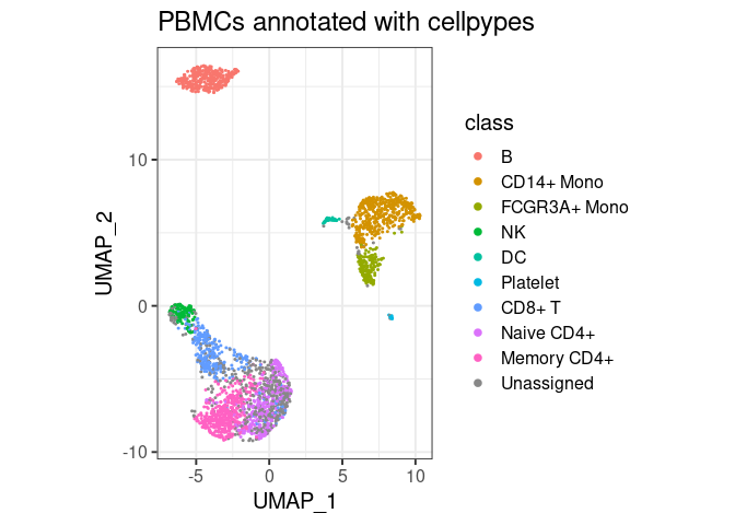
All major cell types are annotated with cell pypes. Note how there are naive CD8+ T cells among the naive CD4 cells. While overlooked in the original tutorial, the marker-based nature of cellpypes revealed this. This is a good example for cellpype’s resolution limit: If UMAP cannot separate cells properly, cellpypes will also struggle – but at least it will be obvious. In practice, one would re-cluster the T cells and try to separate naive CD8+ from naive CD4+, or train a specialized machine learning algorithm to discriminate these two cell types in particular.
cellpypes works with classes defined by gene-based rules.
Whether your classes correspond to biologically relevant cell types is best answered in a passionate discussion on their marker genes you should have with your peers.
Until you are sure, “MS4A1+” is a better class name than “B cell”.
cellpypes uses CP10K (counts per 10 thousand) in functions
rule and feat. This is why and what that
means:
classify,
plot_last and plot_classes leave cells
unassigned if there was not enough evidence.cellpypes compares the expression of a cell and its nearest neighbors to a user-provided threshold, taking the uncertainty due to technical noise into account.
cellpypes assumes a cell’s nearest neighbors are transcriptionally highly similar, so that the technical noise dominates the biological variation. This means that the UMI counts for a given marker gene, say CD3E, came from cells that roughly had the same fraction of CD3E mRNA. We can not use this reasoning to infer the individual cell’s mRNA fraction reliably (which is why imputation introduces artifacts), but we can decide with reasonable confidence whether this cell was at least part of a subpopulation in which many cells expressed this gene highly. In other words:
In cellpypes logic, CD3E+ cells are virtually indistinguishable from cells with high CD3E expression. We just can’t prove they all had CD3E mRNA due to data sparsity.
size
parameter of 100 in R’s pnbinom), as recommended by Lause,
Berens and Kobak (Genome
Biology 2021).K.K with the user-provided threshold
t, because the
sum across NB random variables is again an NB random variable.K are likely to
have come from an NB distribution with rate parameter t*S,
where t is the CP10K threshold supplied through the
rule function, and S is the sum of totalUMI
counts from the cell and its neighbors. If it is very likely, the counts
are too close to the threshold to decide and the cell is left
unassigned. If K lies above the expectancy
t*S, the cell is marked as positive, if below, it is marked
as negative for the given marker gene.t is chosen such that it separates
positive from negative cells, so will typically lie directly between
these two populations. This means that the above procedure should not be
considered a hypothesis test, because t is picked
deliberately to make the null hypothesis (H0: K came from
Pois(t*S)) unlikely.t. If cells were sequenced deeply, S
becomes larger, which means we have more information to decide.The following has a short demo of every function. Let’s say you have
completed the Seurat
pbmc2700 tutorial (or it’s shortcut),
then you can start pyping from this pbmc object:
pbmc <- pype_from_seurat(seurat_object)Visualize marker gene expression with feat (short for
feature plot):
pbmc %>%
  feat(c("NKG7", "MS4A1"))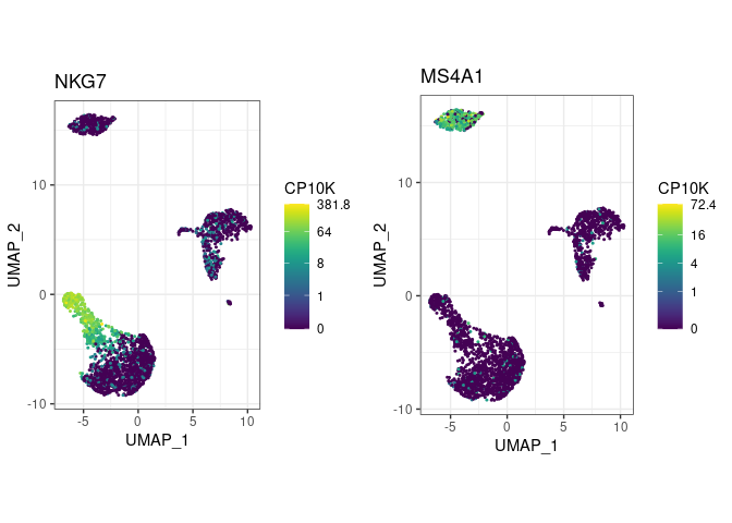
min_dist and
spread parameters. Compute UMAP with spread=5
and you’ll be able to see much more in your embeddings!Create a few cell type rules and plot the most recent
one with plot_last:
pbmc %>%
  rule("CD14+ Mono",  "CD14",    ">", 1)                    %>%
  rule("CD14+ Mono",  "LYZ",     ">", 20)                   %>%
  # uncomment this line to have a look at the LYZ+ rule:
  # plot_last()
  rule("Tcell",       "CD3E",    ">", 3.5)                  %>%
  rule("CD8+ T",      "CD8A",    ">", 1,  parent="Tcell")   %>%
  plot_last()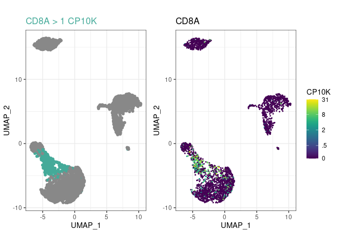
plot_last function plots the last rule you have
added to the object. You can move it between any of the above lines to
look at the preceding rule, as indicated by the commented
plot_last call above.parent argument, to
arbitrary depths. In this example, CD8+ T cells are
CD3E+CD8A+, not just CD8A+, because their
ancestor Tcell had a rule for CD3E.pype_code_template().Get cell type labels with classify or plot them directly
with plot_classes (which wraps ggplot2 code around
classify):
# rules for several cell types:
pbmc2 <- pbmc %>%
  rule("Bcell",       "MS4A1",   ">", 1)                    %>%
  rule("CD14+ Mono",  "CD14",    ">", 1)                    %>%
  rule("CD14+ Mono",  "LYZ",     ">", 20)                   %>%
  rule("Tcell",       "CD3E",    ">", 3.5)                  %>%
  rule("CD8+ T",      "CD8A",    ">", 1,  parent="Tcell")

pbmc2 %>% plot_classes()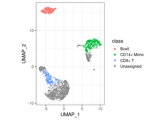
pbmc2 %>% plot_classes(c("Tcell", "CD8+ T")) + ggtitle("T cells")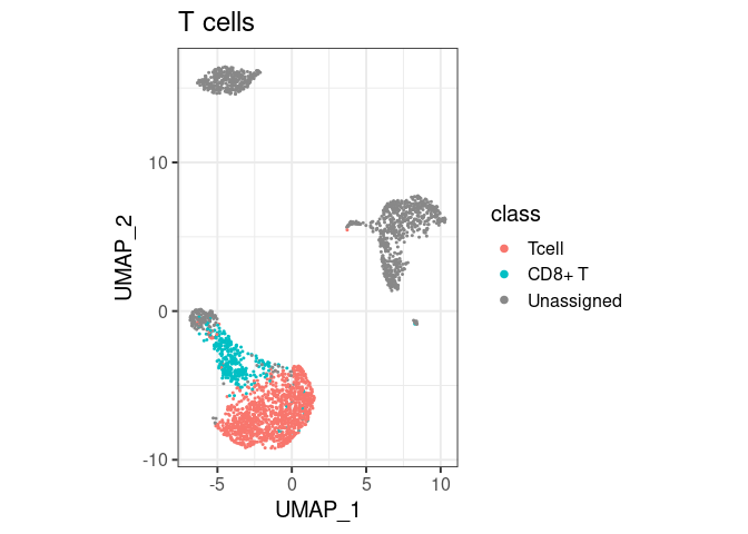
head(classify(pbmc2))
#> AAACATACAACCAC-1 AAACATTGAGCTAC-1 AAACATTGATCAGC-1 AAACCGTGCTTCCG-1
#>       Unassigned            Bcell       Unassigned       Unassigned
#> AAACCGTGTATGCG-1 AAACGCACTGGTAC-1
#>       Unassigned       Unassigned
#> Levels: Bcell CD14+ Mono CD8+ T Unassignedclassify/plot_classes will use
all classes at the end of the hierarchy. T cells are not plotted in the
first example because they are not the end, they have a ‘child’ called
CD8+ T. You can still have them in the same plot, by
specifically asking for plot_classes(c("Tcell", "CD8+ T"))
(second example).classify returns
Unassigned for cells with mutually exclusive labels (such
as Tcell and Bcell).classify("Tcell") or
classify(c("Tcell","Bcell") – the overlap is masked with
Unassigned in this second call, but not in the first.Tcell and CD8+ T), the more detailed
class is returned (CD8+ T).Let’s imagine the PBMC data had multiple patients and treatment conditions (we made them up here for illustraion):
head(pbmc_meta)
#>    patient treatment
#> 1 patient1   treated
#> 2 patient5   treated
#> 3 patient1   control
#> 4 patient1   treated
#> 5 patient2   treated
#> 6 patient4   control
Every row in pbmc_meta corresponds to one cell in the
pbmc object.
With cellpypes, you can directly pipe a given cell type into DESeq2 to create a DESeq2 DataSet (dds) and test it:
library(DESeq2)
dds <- pbmc %>%
  rule("Bcell",   "MS4A1",   ">", 1)     %>%
  rule("Tcell",   "CD3E",    ">", 3.5)   %>%
  class_to_deseq2(pbmc_meta, "Tcell", ~ treatment)
#> converting counts to integer mode
# test for differential expression and get DE genes:
dds <- DESeq(dds)
#> estimating size factors
#> estimating dispersions
#> gene-wise dispersion estimates
#> mean-dispersion relationship
#> final dispersion estimates
#> fitting model and testing
data.frame(results(dds)) %>% arrange(padj) %>% head
#>                  baseMean log2FoldChange     lfcSE         stat    pvalue
#> AL627309.1     0.25114064    -0.46193495 2.2886865 -0.201834087 0.8400464
#> AP006222.2     0.15001429     0.01895508 3.1165397  0.006082093 0.9951472
#> RP11-206L10.2  0.08742633    -0.46193859 3.1165397 -0.148221631 0.8821679
#> LINC00115      0.58340105     0.43747304 1.5879796  0.275490341 0.7829395
#> SAMD11         0.08742633    -0.46193859 3.1165397 -0.148221631 0.8821679
#> NOC2L         12.53882917    -0.57349677 0.3465506 -1.654871847 0.0979505
#>                    padj
#> AL627309.1    0.9998786
#> AP006222.2    0.9998786
#> RP11-206L10.2 0.9998786
#> LINC00115     0.9998786
#> SAMD11        0.9998786
#> NOC2L         0.9998786
In this dummy example, there is no real DE to find because we assigned cells randomly to treated/control.
Instead of piping into DESeq2 directly, you can also form pseudobulks
with pseudobulk and helper function
pseudobulk_id. This can be applied to any single-cell count
data, independent from cellpypes. For example, counts could
be seurat@assays$RNA@counts and meta_df could
be selected columns from seurat@meta.data.
pbmc3 <- pbmc %>% rule("Tcell",   "CD3E",    ">", 3.5)
is_class <- classify(pbmc3) == "Tcell"
counts <- pseudobulk(pbmc$raw[,is_class],
                     pseudobulk_id(pbmc_meta[is_class,]))
counts[35:37, 1:3]
#> 3 x 3 Matrix of class "dgeMatrix"
#>            patient1.control patient1.treated patient2.control
#> AL645608.1                0                0                0
#> NOC2L                    13                6               16
#> KLHL17 0 0 0Yes. Do it. You can search
similar problems or create new issues on gitHub. If you want to be
nice and like fast help for free, try to provide a minimal
example of your problem if possible. Make sure to include the
version of your cellpypes installation, obtained e.g. with
packageVersion("cellpypes").
Unassigned cells (grey) are not necessarily bad but a way to respect the signal-to-noise limit. Unassigned cells arise for two reasons:
Unassigned, but this behavior can be controlled with the
replace_overlap_with argument in classify and
plot_classes.In cellpypes logic, Differential Expression (DE) analysis refers to comparing multiple samples (patients/mice/…) from at least two different groups (control/treated/…). These so called multi-condition multi-sample comparisons have individuals, not cells, as unit of replication, and give reliable p-values.
Finding cluster markers, in contrast, is circular and results in invalid p-values (which are useful for ranking marker genes, not for determining significance). The circularity comes from first using gene expression differences to find clusters, and then testing the null hypothesis that the same genes have no differences between clusters.
Pseudobulk approaches have been shown to perform as advertised, while many single-cell methods do not adjust p-values correctly and fail to control the false-discovery rate. Note that DESeq2, however, requires you to filter out lowly expressed genes.