![]()
![]()
The goal of bigtime is to sparsely estimate large time
series models such as the Vector AutoRegressive (VAR) Model, the Vector
AutoRegressive with Exogenous Variables (VARX) Model, and the Vector
AutoRegressive Moving Average (VARMA) Model. The univariate cases are
also supported.
The package can be installed from CRAN using
install.packages("bigtime")You can install the development version (= the latest version) of bigtime from github as follows:
# install.packages("devtools")
devtools::install_github("ineswilms/bigtime")bigtime comes with example data sets created from a VAR, VARMA and
VARX DGP. These data sets are called var.example,
varma.example, and varx.example respectively
and can be loaded into the environment by calling
data(var.example) and similarly for the others. We can have
a look at the varx.example data set by first loading it
into the environment and then, using a little utility function, plotting
it.
library(bigtime)
suppressMessages(library(tidyverse)) # Will be used for nicer visualisations
#> Warning: package 'tidyverse' was built under R version 4.0.5
#> Warning: package 'ggplot2' was built under R version 4.0.3
#> Warning: package 'readr' was built under R version 4.0.4
#> Warning: package 'purrr' was built under R version 4.0.3
#> Warning: package 'dplyr' was built under R version 4.0.5
#> Warning: package 'stringr' was built under R version 4.0.3
#> Warning: package 'forcats' was built under R version 4.0.4
data(varx.example) # loading the varx example data


plot_series <- function(Y){
  as_tibble(Y) %>%
  mutate(Time = 1:n()) %>%
  pivot_longer(-Time, names_to = "Series", values_to = "vals") %>%
  mutate(Series = factor(Series, levels = colnames(Y))) %>%
  ggplot() +
  geom_line(aes(Time, vals)) +
  facet_wrap(facets = vars(Series), ncol = 1) +
  ylab("") +
  theme_bw()
}

plot_series(Y.varx)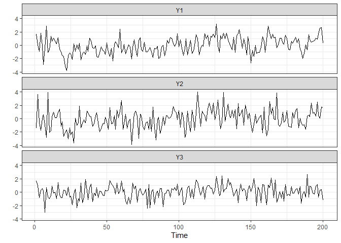
plot_series(X.varx)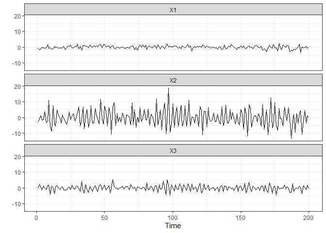
While we could use the example data provided, bigtime also
supports simulation of VAR models using both lasso and elementwise type
sparsity patterns. Since lasso is the most widely known one, we will
start off with lasso. To simulate a VAR model having lasso type of
sparsity, use the simVAR function and set
sparsity_pattern="lasso". The lasso sparsity pattern has
the additional num_zero option which determines the number
of zeros in the VAR coefficient matrix (excluding intercepts). Note:
we also set a seed so that the simulation is replicable. We can
then use the summary function to obtain a summary of the
simulated data.
periods <- 200 # time series length
k <- 5 # number of time series
p <- 8 # maximum lag
sparsity_options <- list(num_zero = 15) # 15 zeros across the k=5 VAR coefficient matrices
sim_data <- simVAR(periods = periods, k = k, p = p,
                   sparsity_pattern = "lasso",
                   sparsity_options = sparsity_options,
                   seed = 123456,
                   decay = 0.01) # the smaller decay the larger early coefs w.r.t. to later ones
Y.lasso <- sim_data$Y
summary(sim_data) # obtaining a summary of the simulated time series data
#> #### General Information ####
#>
#> Seed                                        123456
#> Time series length                          200
#> Burnin                                      200
#> Variables Simulated                         5
#> Number of Lags                              8
#> Coefficients were randomly created?         TRUE
#> Maximum Eigenvalue of Companion Matrix      0.8
#> Sparsity Pattern                            lasso
#>
#>
#> #### Sparsity Options ####
#>
#> $num_zero
#> [1] 15
#>
#>
#>
#> #### Coefficient Matrix ####
#>
#>                  Y1            Y2            Y3            Y4            Y5
#> Y1.L1  3.344178e-01 -1.107252e-01 -1.423944e-01  3.509198e-02  9.033998e-01
#> Y2.L1  3.347094e-01  5.264215e-01  1.003833e+00  4.685881e-01 -1.709388e-01
#> Y3.L1 -3.995565e-01 -4.468152e-01 -2.235442e-02  4.710753e-01  4.224553e-01
#> Y4.L1  2.310627e-02 -2.948322e-01  3.732432e-01  6.691342e-01  2.244958e-01
#> Y5.L1  0.000000e+00  5.040150e-01  1.543970e-02  7.602611e-02  1.855509e-01
#> Y1.L2 -1.714191e-03  6.652793e-05  2.827333e-03  3.898174e-03 -2.488847e-03
#> Y2.L2 -3.432958e-03  2.790046e-04 -4.196394e-03 -1.102596e-02 -4.531967e-03
#> Y3.L2 -3.456294e-03  6.257595e-03  4.071610e-03  4.187554e-03 -4.475995e-03
#> Y4.L2  0.000000e+00  3.882016e-03  6.860267e-04 -3.594939e-03  6.349122e-04
#> Y5.L2 -2.013360e-03  0.000000e+00 -4.561977e-04  4.355841e-03 -4.860029e-03
#> Y1.L3 -7.090490e-05 -1.972221e-05  1.289428e-05  0.000000e+00  0.000000e+00
#> Y2.L3 -1.362040e-05 -4.321743e-05 -5.979591e-05 -1.013789e-05 -4.890420e-06
#> Y3.L3 -2.603130e-05  1.255775e-05  4.926041e-06 -3.356641e-05  2.408345e-05
#> Y4.L3 -9.864658e-06 -7.407063e-06  9.288386e-07 -1.943981e-05 -2.959808e-05
#> Y5.L3  5.224473e-05  2.264257e-05 -7.240193e-05  1.758216e-05 -5.780336e-05
#> Y1.L4  3.821882e-07 -2.899947e-07  1.955819e-08 -6.271466e-07 -9.234996e-07
#> Y2.L4  4.644695e-07 -2.826756e-07 -6.312740e-07  2.079154e-07 -4.271531e-07
#> Y3.L4  1.887393e-08  3.401594e-07  1.735509e-07  2.097019e-07  0.000000e+00
#> Y4.L4 -1.992917e-07  5.054378e-07  2.266186e-07 -1.382372e-07  2.907276e-07
#> Y5.L4  3.465950e-07  1.481081e-07  6.351945e-07  2.421511e-08  5.162710e-08
#> Y1.L5 -3.412591e-09  4.406386e-09 -4.838797e-09  2.333901e-09  3.464337e-09
#> Y2.L5  3.943109e-09 -5.099138e-09 -4.262808e-12 -3.854296e-09  5.050800e-09
#> Y3.L5 -3.476037e-09  9.989383e-10 -3.456284e-10 -1.977003e-09 -1.078979e-09
#> Y4.L5 -1.601388e-09 -3.787661e-09  4.063988e-09 -1.639348e-09 -7.263552e-10
#> Y5.L5  4.748150e-09 -6.451814e-09 -9.114958e-09 -8.185059e-09 -2.599211e-09
#> Y1.L6  2.878848e-11 -4.147466e-12  0.000000e+00 -3.921230e-11  0.000000e+00
#> Y2.L6  1.757755e-12 -4.097641e-11  3.182509e-11  2.012060e-11 -6.235119e-11
#> Y3.L6  3.543788e-11 -8.333751e-12  7.345804e-11  7.110232e-12 -3.232298e-11
#> Y4.L6  7.813330e-11  4.861321e-12 -1.423732e-11  4.223140e-11  4.665353e-11
#> Y5.L6 -3.204189e-11  3.110420e-11 -8.002152e-11 -1.406136e-11  1.527682e-11
#> Y1.L7  1.035718e-13  3.868736e-13  0.000000e+00  3.274603e-14 -6.488767e-14
#> Y2.L7  5.105382e-13 -2.889064e-13  6.181295e-13  3.424112e-13  3.218496e-13
#> Y3.L7 -1.374288e-13  4.027135e-14  6.096383e-14  0.000000e+00 -1.371909e-13
#> Y4.L7 -5.274508e-13 -7.661388e-13  2.324513e-13 -6.879730e-13  0.000000e+00
#> Y5.L7 -6.332500e-13  7.399670e-13  3.913858e-13 -1.324464e-13  4.786837e-13
#> Y1.L8 -1.337775e-15  6.673161e-16  0.000000e+00  7.885634e-15  2.243677e-15
#> Y2.L8 -2.573135e-15 -1.884193e-16  4.549152e-15  1.160132e-15  1.854712e-15
#> Y3.L8  4.740580e-15  0.000000e+00 -2.501340e-15 -2.635646e-15  2.839144e-15
#> Y4.L8  0.000000e+00 -1.797436e-15  4.488466e-15  7.460492e-16 -1.452254e-15
#> Y5.L8  9.907469e-16  1.438249e-15  6.791980e-17 -9.437176e-16  0.000000e+00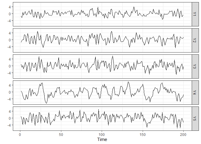
A VAR with HLag (elementwise) type of sparsity can be simulated using
simVAR and by setting sparsity_pattern="HLag".
Three extra options exist: (1) zero_min determines the
minimum number of zero coefficients of each variable in each equation,
(2) zero_max determines the maximum number of zero
coefficients of each variable in each equation, and (3)
zeroes_in_self is a boolean option that if TRUE, zero
coefficients of the ith variable can exist in the ith
equation.
periods <- 200
k <- 5 # Number of time series
p <- 5 # Maximum lag
sparsity_options <- list(zero_min = 0,
                         zero_max = 5,
                         zeroes_in_self = TRUE)
sim_data <- simVAR(periods = periods, k = k, p = p,
                   sparsity_pattern = "HLag",
                   sparsity_options = sparsity_options,
                   seed = 123456,
                   decay = 0.01)
Y.hlag <- sim_data$Y
summary(sim_data) # Obtaining a summary of the simulation
#> #### General Information ####
#>
#> Seed                                        123456
#> Time series length                          200
#> Burnin                                      200
#> Variables Simulated                         5
#> Number of Lags                              5
#> Coefficients were randomly created?         TRUE
#> Maximum Eigenvalue of Companion Matrix      0.8
#> Sparsity Pattern                            hvar
#>
#>
#> #### Sparsity Options ####
#>
#> $zero_min
#> [1] 0
#>
#> $zero_max
#> [1] 5
#>
#> $zeroes_in_self
#> [1] TRUE
#>
#>
#>
#> #### Coefficient Matrix ####
#>
#>                  Y1            Y2            Y3            Y4            Y5
#> Y1.L1  0.000000e+00 -1.032031e-01 -1.327209e-01  3.270802e-02  8.420276e-01
#> Y2.L1  3.119710e-01  4.906592e-01  9.356382e-01  4.367547e-01 -1.593261e-01
#> Y3.L1 -3.724128e-01 -4.164610e-01 -2.083578e-02  4.390729e-01  3.937560e-01
#> Y4.L1  2.153655e-02 -2.748029e-01  3.478871e-01  0.000000e+00  2.092447e-01
#> Y5.L1 -2.818808e-01  4.697750e-01  1.439081e-02  7.086130e-02  1.729456e-01
#> Y1.L2  0.000000e+00  0.000000e+00  2.635259e-03  3.633353e-03 -2.319768e-03
#> Y2.L2 -3.199742e-03  2.600505e-04  0.000000e+00 -1.027691e-02 -4.224090e-03
#> Y3.L2 -3.221492e-03  5.832487e-03  0.000000e+00  3.903074e-03 -4.171920e-03
#> Y4.L2  0.000000e+00  3.618292e-03  6.394217e-04  0.000000e+00  5.917797e-04
#> Y5.L2 -1.876583e-03 -3.611195e-03 -4.252061e-04  4.059929e-03 -4.529864e-03
#> Y1.L3  0.000000e+00  0.000000e+00  1.201831e-05  0.000000e+00  5.747130e-05
#> Y2.L3 -1.269510e-05 -4.028146e-05  0.000000e+00 -9.449180e-06 -4.558191e-06
#> Y3.L3 -2.426287e-05  1.170464e-05  0.000000e+00 -3.128609e-05  2.244735e-05
#> Y4.L3  0.000000e+00  0.000000e+00  0.000000e+00  0.000000e+00 -2.758734e-05
#> Y5.L3  0.000000e+00  2.110436e-05 -6.748333e-05  1.638772e-05 -5.387651e-05
#> Y1.L4  0.000000e+00  0.000000e+00  1.822951e-08  0.000000e+00 -8.607620e-07
#> Y2.L4  4.329159e-07 -2.634722e-07  0.000000e+00  0.000000e+00 -3.981346e-07
#> Y3.L4  0.000000e+00  3.170507e-07  0.000000e+00  1.954558e-07 -9.491777e-08
#> Y4.L4  0.000000e+00  0.000000e+00  0.000000e+00  0.000000e+00  0.000000e+00
#> Y5.L4  0.000000e+00  1.380464e-07  5.920428e-07  0.000000e+00  4.811983e-08
#> Y1.L5  0.000000e+00  0.000000e+00  0.000000e+00  0.000000e+00  3.228988e-09
#> Y2.L5  0.000000e+00  0.000000e+00  0.000000e+00  0.000000e+00  0.000000e+00
#> Y3.L5  0.000000e+00  0.000000e+00  0.000000e+00 -1.842696e-09 -1.005678e-09
#> Y4.L5  0.000000e+00  0.000000e+00  0.000000e+00  0.000000e+00  0.000000e+00
#> Y5.L5  0.000000e+00 -6.013512e-09 -8.495736e-09  0.000000e+00  0.000000e+00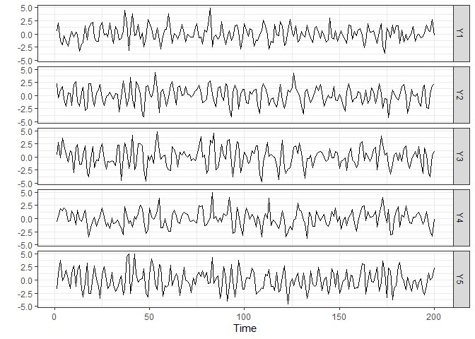
The above simulated data (and truly any other data) could then be
estimated using an L1-penalty (lasso penalty) on the autoregressive
coefficients. To this end, set the VARpen argument in the
sparseVAR function equal to L1. Note: it is recommended
to standardise the data. Bigtime will give a warning if the data is not
standardised but will not stop you from continuing. Setting
selection="none", the default, allows us to specify the
penalization we want. Furthermore, we can predefine the maximum
lag-order by changing the p argument to the desired value.
However, we do not recommend this, as the bigtime will, by default,
choose a maximum lag-order that is well suited in many scenarios.
VAR.L1 <- sparseVAR(Y = scale(Y.lasso), # standardising the data
                    VARpen = "L1", # using lasso penalty
VARlseq = 1.5) # Specifying the penalty to be used. selection="none" is the default.For the selection of the penalization parameter, we can either set
the selection argument to "none", which would
return a model for a sequence of penalizations, or use time series
cross-validation by setting selection="cv", or finally we
could also use any of BIC, AIC, or HQ information criteria by setting
the selection arguments to any of "bic",
"aic", or "hq" respectively. We will start of
by using time series cross-validation and will therefore set
selection="cv". The default is to use a cross-validation
score based on one-step ahead predictions but you can change the default
forecast horizon under the argument h.
VAR.L1 <- sparseVAR(Y=scale(Y.lasso),  # standardising the data
                   selection = "cv", # using time series cross-validation
                   VARpen = "L1") # using the lasso penalty
The plot_cv function can be used to investigate the
cross-validation procedure. The returned plot shows the mean MSFE for
each penalization together with error bars for plus-minus one standard
deviation. The black dashed line indicates the penalty parameter choice
that lead to the smallest MSFE in the CV procedure. The red dotted line,
on the other hand, shows the one-standard-error solution. It picks the
most parsimonious model within one standard error of the best
cross-validation score. The latter is the one that is chosen by default
in sparseVAR.
plot_cv(VAR.L1)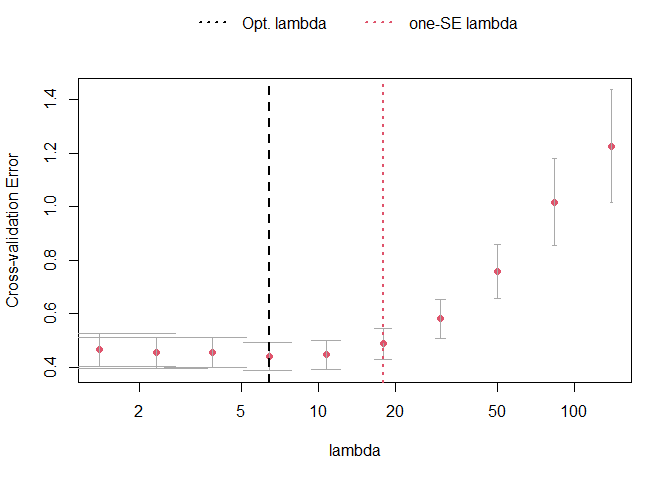
Further investigation into the model can be done by using the
function lagmatrix, which returns the lagmatrix of the
estimated autoregressive coefficients. If entry
(i, j) = x, this means that the sparse
estimator indicates the effect of time series j on time series
i to last for x periods. Setting the
returnplot argument to TRUE will return a
heatmap for better visual inspection.
LhatL1 <- lagmatrix(fit=VAR.L1, returnplot=TRUE)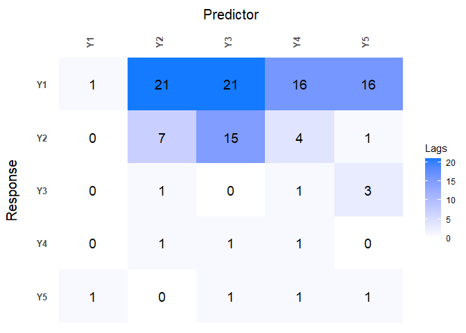
The lag matrix is typically sparse as it contains some empty (i.e., zero) cells. However, VAR models estimated with a standard L1-penalty are typically not easily interpretable as they select many high lag order coefficients (i.e., large values in the lagmatrix).
To circumvent this problem, we advise using a lag-based
hierarchically sparse estimation procedure, which boils down to using
the default option HLag for the VARpen argument. This
estimation procedure encourages low maximum lag orders, often results in
sparser lagmatrices, and hence more interpretable models.
Models can be estimated using the hierarchical penalization by using
the default argument to VARpen, namely HLag.
Model selection can again be done by either setting
selection="none" and obtaining a whole sequence of models,
or by using any of cv, bic, aic, hq.
VARHLag_none <- sparseVAR(Y=scale(Y.hlag),
                          selection = "none") # HLag is the default VARpen option
VARHLag_cv <- sparseVAR(Y=scale(Y.hlag),
                        selection = "cv")
VARHLag_bic <- sparseVAR(Y=scale(Y.hlag),
                         selection = "bic") # This will also give a table for IC comparison showing the selected lambda for each IC
#>
#>
#> #### Selected the following lambda ####
#>
#>      AIC      BIC       HQ
#> 10.74023 10.74023 10.74023
#>
#>
#> #### Details ####
#>
#>      lambda         AIC         BIC          HQ
#> 1  138.7154     -0.9793     -0.9793     -0.9793
#> 2   83.1577     -1.7792     -1.6473     -1.7258
#> 3   49.8517     -3.0055     -2.7746      -2.912
#> 4   29.8853     -4.1453     -3.8155     -4.0118
#> 5   17.9158      -4.826     -4.4631     -4.6791
#> 6   10.7402 ==> -5.0769 ==> -4.6151   ==> -4.89
#> 7    6.4386     -5.0698     -4.3277     -4.7695
#> 8    3.8598     -4.6703     -3.0377     -4.0096
#> 9    2.3139     -2.7531      2.5737     -0.5974
#> 10 1.3872 -1.5512 6.5956 1.7457Depending on which selection procedure was used, various diagnostics
can be produced. Former and foremost, all selection procedures support
the fitted and residuals functions to obtain
the fitted and residual values respectively. Both functions return a 3D
array if the model used selection="none" corresponding to
the fitted/residual values for each model in the penalization
sequence.
res_VARHLag_none <- residuals(VARHLag_none) # This is a 3D array
dim(res_VARHLag_none)
#> [1] 179   5  10
When an actual selection method was used
(cv, bic, aic, hq), then other diagnostic functions exist.
For cv, plot_cv could be used again, just as
shown above. For all, the diagnostics_plot function can be
used to obtain a plot of fitted and residual values.
p_bic <- diagnostics_plot(VARHLag_bic, variable = "Y3") # variable argument can be numeric or character
p_cv <- diagnostics_plot(VARHLag_cv, variable = "Y3") # variable argument can be numeric or character

plot(p_bic)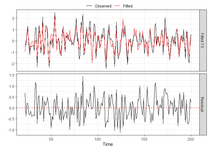
plot(p_cv)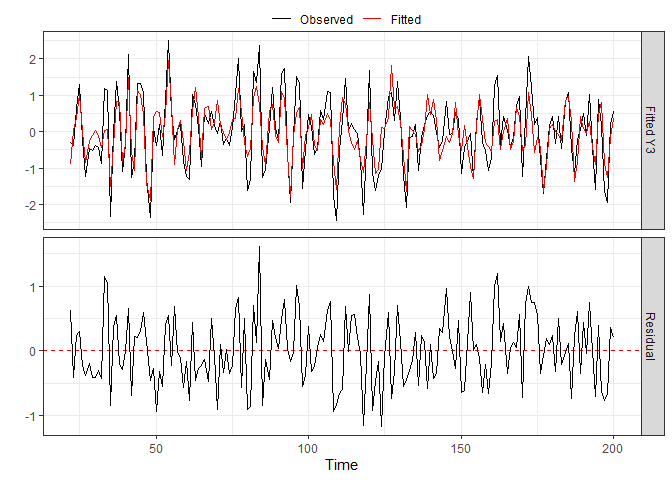
Often practitioners are interested in incorporating the impact of
unmodeled exogenous variables (X) into the VAR model. To do this, you
can use the sparseVARX function which has an argument
X where you can enter the data matrix of exogenous time
series. For demonstration purposes, we will use the
varx.example data set that is part of bigtime.
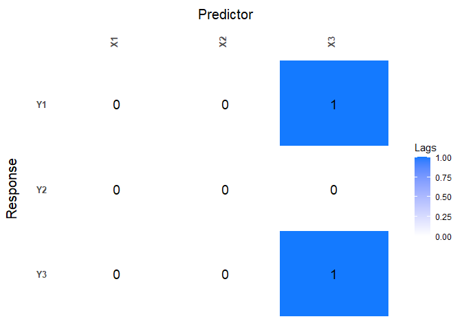
data(varx.example)When applying the lagmatrix function to an estimated
sparse VARX model, the lag matrices of both the endogenous and exogenous
autoregressive coefficients are returned.
sparseVARX supports the same selection
arguments as sparseVAR:
none, cv, bic, aic, hq, and it is again recommended to
standardise the data.
VARXfit_cv <- sparseVARX(Y=scale(Y.varx), X=scale(X.varx), selection = "cv")
LhatVARX <- lagmatrix(fit=VARXfit_cv, returnplot=TRUE)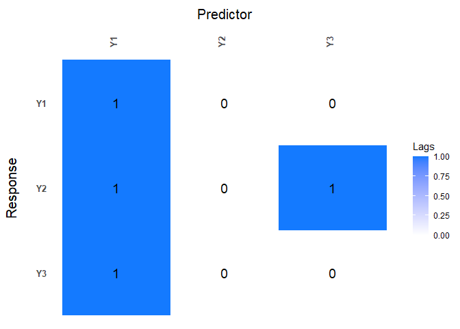
VARX models also support plot_cv if estimated using CV.
The returned plot shows the mean MSFE for each combination of
penalizations in a heatmap. The x-axis show the penalizations for the
exogenous variables, and the y-axis shows the penalizations for the
endogenous variables. The big black dot in the plot below indicates the
one-SE optimal choice, while the contours indicate the mean MSFE in the
CV procedure. The red colour indicates a high MSFE, and light-yellow to
yellow regions indicate low MSFEs.
plot_cv(VARXfit_cv)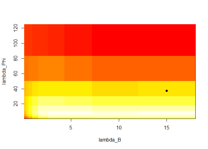
If selection="none" a 3D array will be returned again.
Although not mentioned previously, when setting selection
to none, or any of the IC, one can also easily provide a
penalization sequence, or even just ask for a single penalization
setting. For example, below we intentionally choose a single, small
penalization for the exogenous variables.
VARXfit_none <- sparseVARX(Y=scale(Y.varx), X=scale(X.varx), VARXlBseq = 0.001, selection = "none")
dim(VARXfit_none$Phihat) # This is a 3D array
#> [1]  3 63 10
# This is also 3D but third dimension is equal to ten
# --> one penalization was chosen for B and 10 automatically for Phi
# --> Cross product makes 10
dim(VARXfit_none$Bhat)
#> [1]  3 63 10
Other functions such as residuals, fitted,
and diagnostics_plot are also supported.
VARMA models generalise VAR models and often allow for more
parsimonious representations of the data generating process. To estimate
a VARMA model to a multivariate time series data set, use the function
sparseVARMA, and choose a desired selection method. The
sparse VARMA estimation procedures consists of two stages: in the first
stage a VAR model is estimated from which the residuals are retrieved.
In the second stage these residuals are used as approximated error terms
to estimate the VARMA model. As a default, sparseVARMA uses
CV in the first stage and none in the second stage.
The first stage does not support none: A selection
needs to be made.
Now lag matrices are obtained for the autoregressive (AR) coefficients and the moving average (MAs) coefficients.
data(varma.example)
VARMAfit <- sparseVARMA(Y=scale(Y.varma), VARMAselection = "cv") # VARselection="cv" as default.
LhatVARMA <- lagmatrix(fit=VARMAfit, returnplot=T)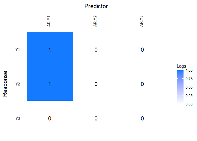
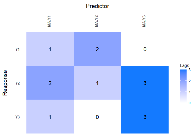
Other functions such as plot_cv, residuals,
fitted and diagnosticsplot are also
supported.
To obtain forecasts from the estimated models, you can use the
directforecast function for VAR, VARMA, and VARX, or the
recursiveforecast function for VAR models. The default
forecast horizon (argument h) is set to one such that
one-step ahead forecasts are obtained, but you can specify your desired
forecast horizon.
Finally, we compare the forecast accuracy of the different models by
comparing their forecasts to the actual time series values of the
var.example data set that comes with bigtime. We will
estimate all models using CV.
In this example, the VARMA model has the best forecast performance (i.e., lowest mean squared prediction error). This is somewhat surprising given the data comes from a VAR model.
data(var.example)
dim(Y.var)
#> [1] 200   5
Y <- Y.var[-nrow(Y.var), ] # leaving the last observation for comparison
Ytest <- Y.var[nrow(Y.var), ]

VARcv <- sparseVAR(Y = scale(Y), selection = "cv")
VARMAcv <- sparseVARMA(Y = scale(Y), VARMAselection = "cv")

Y <- Y.var[-nrow(Y.var), 1:3] # considering first three variables as endogenous
X <- Y.var[-nrow(Y.var), 4:5] # and last two as exogenous
VARXcv <- sparseVARX(Y = scale(Y), X = scale(X), selection = "cv")

VARf <- directforecast(VARcv) # default is h=1
VARXf <- directforecast(VARXcv)
VARMAf <- directforecast(VARMAcv)

# We can only compare forecasts for the first three variables
# because VARX models only forecast endogenously modelled variables
mean((VARf[1:3]-Ytest[1:3])^2)
#> [1] 0.6252039
mean((VARXf[1:3]-Ytest[1:3])^2)
#> [1] 0.6319843
mean((VARMAf[1:3]-Ytest[1:3])^2) # lowest=best
#> [1] 0.4571325
Note that we could easily obtain longer horizon forecasts for the VAR
model by using the recursiveforecast function. It is
recommended to call is.stable first though, to check
whether the obtained VAR model is stable.
is.stable(VARcv)
#> [1] TRUE
rec_fcst <- recursiveforecast(VARcv, h = 10)
plot(rec_fcst, series = "Y2", last_n = 50) # Plotting of a recursive forecast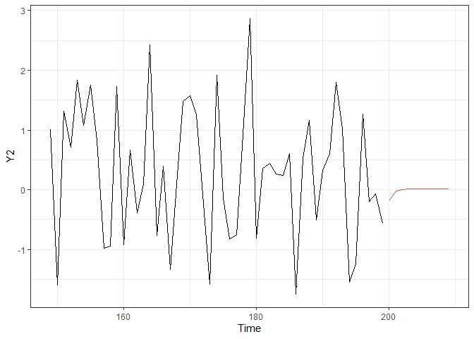
The functions sparseVAR, sparseVARX,
sparseVARMA can also be used for the univariate setting
where the response time series Y is univariate. Below we
illustrate the usefulness of the sparse estimation procedure as
automatic lag selection procedures.
We start by generating a time series of length n = 50 from a
stationary AR model and by plotting it. The sparseVAR
function can also be used in the univariate case as it allows the
argument Y to be a vector.
The lagmatrix function gives the selected autoregressive
order of the sparse AR model. The true order is one.
periods <- 50
k <- 1
p <- 1
sim_data <- simVAR(periods, k, p,
                   sparsity_pattern = "none",
                   max_abs_eigval = 0.5,
                   seed = 123456)
summary(sim_data)
#> #### General Information ####
#>
#> Seed                                        123456
#> Time series length                          50
#> Burnin                                      50
#> Variables Simulated                         1
#> Number of Lags                              1
#> Coefficients were randomly created?         TRUE
#> Maximum Eigenvalue of Companion Matrix      0.5
#> Sparsity Pattern                            none
#>
#>
#> #### Sparsity Options ####
#>
#> NULL
#>
#>
#> #### Coefficient Matrix ####
#>
#>           [,1]
#> [1,] 0.4998982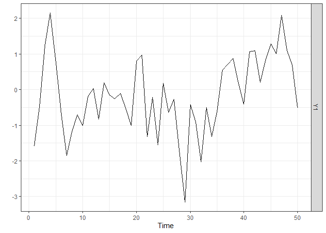
y <- scale(sim_data$Y)
ARfit <- sparseVAR(Y=y, selection = "cv")
lagmatrix(ARfit)
#> $LPhi
#>      [,1]
#> [1,]    1
Note that all diagnostics functions discussed for the VAR, VARMA, VARX cases also work for univariate cases; so do the forecasting functions.
We start by generating a time series of length n = 50 from a
stationary ARX model and by plotting it. The sparseVARX
function can also be used in the univariate case as it allows the
arguments Y and X to be vectors. The
lagmatrix function gives the selected endogenous (under
LPhi) and exogenous autoregressive (under LB)
orders of the sparse ARX model. The true orders are one.
periods <- 50
k <- 1
p <- 1
burnin <- 100
Xsim <- simVAR(periods+burnin+1, k, p, max_abs_eigval = 0.8, seed = 123)
edist <- lag(Xsim$Y)[-1, ] + rnorm(periods + burnin, sd = 0.1)
Ysim <- simVAR(periods, k , p, max_abs_eigval = 0.5, seed = 789,
               e_dist = t(edist), burnin = burnin)
plot(Ysim)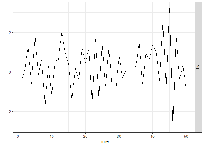
x <- scale(Xsim$Y[-(1:(burnin+1))])
y <- scale(Ysim$Y)

ARXfit <- sparseVARX(Y=y, X=x, selection = "cv")
lagmatrix(fit=ARXfit)
#> $LPhi
#>      [,1]
#> [1,]    1
#>
#> $LB
#>      [,1]
#> [1,] 2We start by generating a time series of length n = 50 from a
stationary ARMA model and by plotting it. The sparseVARMA
function can also be used in the univariate case as it allows the
argument Y to be a vector. The lagmatrix
function gives the selected autoregressive (under LPhi) and
moving average (under LTheta) orders of the sparse ARMA
model. The true orders are one.
periods <- 50
k <- 1
p.u <- 1
p.y <- 1
burnin <- 100

u <- rnorm(periods + 1 + burnin, sd = 0.1)
u <- embed(u, dimension = p.u + 1)
u <- u * matrix(rep(c(1, 0.2), nrow(u)), nrow =  nrow(u), byrow = TRUE) # Second column is lagged, first is current error
edist <- rowSums(u)

Ysim <- simVAR(periods, k, p, e_dist = t(edist),
               max_abs_eigval = 0.5, seed = 789,
               burnin = burnin)
summary(Ysim)
#> #### General Information ####
#>
#> Seed                                        789
#> Time series length                          50
#> Burnin                                      100
#> Variables Simulated                         1
#> Number of Lags                              1
#> Coefficients were randomly created?         TRUE
#> Maximum Eigenvalue of Companion Matrix      0.5
#> Sparsity Pattern                            none
#>
#>
#> #### Sparsity Options ####
#>
#> NULL
#>
#>
#> #### Coefficient Matrix ####
#>
#>           [,1]
#> [1,] 0.4989384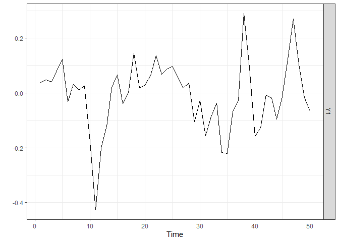
ARMAfit <- sparseVARMA(Y=y, VARMAselection = "cv")
lagmatrix(fit=ARMAfit)
#> $LPhi
#>      [,1]
#> [1,]    3
#>
#> $LTheta
#>      [,1]
#> [1,] 0For a non-technical introduction to VAR models see this interactive notebook and for an interactive notebook demonstrating the use of bigtime for high-dimensional VARs, see this notebook. Note: Loading these notebooks sometimes can take quite some time. Please be patient or try another time.
Nicholson William B., Wilms Ines, Bien Jacob and Matteson David S. (2020), “High-dimensional forecasting via interpretable vector autoregression”, Journal of Machine Learning Research, 21(166), 1-52.
Wilms Ines, Basu Sumanta, Bien Jacob and Matteson David S. (2021), “Sparse Identification and Estimation of Large-Scale Vector AutoRegressive Moving Averages”, Journal of the American Statistical Association, doi: 10.1080/01621459.2021.1942013.
Wilms Ines, Basu Sumanta, Bien Jacob and Matteson David S. (2017), “Interpretable Vector AutoRegressions with Exogenous Time Series”, NIPS 2017 Symposium on Interpretable Machine Learning, arXiv:1711.03623