![]()
![]()
Accumulated Local Effects (ALE) were initially developed as a model-agnostic approach for global explanations of the results of black-box machine learning algorithms (Apley, Daniel W., and Jingyu Zhu. ‘Visualizing the effects of predictor variables in black box supervised learning models.’ Journal of the Royal Statistical Society Series B: Statistical Methodology 82.4 (2020): 1059-1086 doi:10.1111/rssb.12377). ALE has two primary advantages over other approaches like partial dependency plots (PDP) and SHapley Additive exPlanations (SHAP): its values are not affected by the presence of interactions among variables in a model and its computation is relatively rapid. This package reimplements the algorithms for calculating ALE data and develops highly interpretable visualizations for plotting these ALE values. It also extends the original ALE concept to add bootstrap-based confidence intervals and ALE-based statistics that can be used for statistical inference.
For more details, see Okoli, Chitu. 2023. “Statistical Inference Using Machine Learning and Classical Techniques Based on Accumulated Local Effects (ALE).” arXiv. doi:10.48550/arXiv.2310.09877.
The {ale} package defines four main {S7}
classes:
ALE: data for 1D ALE (single variables) and 2D ALE
(two-way interactions). ALE values may be bootstrapped with ALE
statistics calculated.ModelBoot: bootstrap results an entire model, not just
the ALE values. This function returns the bootstrapped model statistics
and coefficients as well as the bootstrapped ALE values. This is the
appropriate approach for models that have not been cross-validated.ALEPlots: store ALE plots generated from either
ALE or ModelBoot with convenient
print(), plot(), and get()
methods.ALEpDist: a distribution object for calculating the
p-values for the ALE statistics of an ALE object.You can obtain direct help for any of the package’s user-facing
functions with the R help() function, e.g.,
help(ale). However, the most detailed documentation is
found in the website
for the most recent development version. There you can find
several articles. We particularly recommend:
You can obtain the official releases from CRAN:
install.packages('ale')The CRAN releases are extensively tested and should have relatively
few bugs. However, this package is still in beta stage. For the
{ale} package, that means that there will occasionally be
new features with changes in the function interface that might break the
functionality of earlier versions. Please excuse us for this as we move
towards a stable version that flexibly meets the needs of the broadest
user base.
To get the most recent features, you can install the development version of the package from GitHub with:
# install.packages('pak')
pak::pak('tripartio/ale')
The development version in the main branch of GitHub is always thoroughly checked. However, the documentation might not be fully up-to-date with the functionality.
We will give two demonstrations of how to use the package: first, a simple demonstration of ALE plots, and second, a more sophisticated demonstration suitable for statistical inference with p-values. For both demonstrations, we begin by fitting a GAM model. We assume that this is a final deployment model that needs to be fitted to the entire dataset.
library(dplyr)
#>
#> Attaching package: 'dplyr'
#> The following objects are masked from 'package:stats':
#>
#>     filter, lag
#> The following objects are masked from 'package:base':
#>
#>     intersect, setdiff, setequal, union

# Load diamonds dataset with some cleanup
diamonds <- ggplot2::diamonds |>
  filter(!(x == 0 | y == 0 | z == 0)) |>
  # https://lorentzen.ch/index.php/2021/04/16/a-curious-fact-on-the-diamonds-dataset/
  distinct(
    price, carat, cut, color, clarity,
    .keep_all = TRUE
  ) |>
  rename(
    x_length = x,
    y_width = y,
    z_depth = z,
    depth_pct = depth
  )
# Create a GAM model with flexible curves to predict diamond price
# Smooth all numeric variables and include all other variables
# Build the model on training data, not on the full dataset.
gam_diamonds <- mgcv::gam(
  price ~ s(carat) + s(depth_pct) + s(table) + s(x_length) + s(y_width) + s(z_depth) +
    cut + color + clarity,
  data = diamonds
)For the simple demonstration, we directly create ALE data with the
ALE() function and then plot the ggplot plot
objects.
library(ale)
#>
#> Attaching package: 'ale'
#> The following object is masked from 'package:base':
#>
#>     get

# For speed, these examples use retrieve_rds() to load pre-created objects
# from an online repository.
# To run the code yourself, execute the code blocks directly.
serialized_objects_site <- "https://github.com/tripartio/ale/raw/main/download"

# Create ALE data
ale_gam_diamonds <- retrieve_rds(
  # For speed, load a pre-created object by default.
  c(serialized_objects_site, 'ale_gam_diamonds.0.5.2.rds'),
  {
    # To run the code yourself, execute this code block directly.
    ALE(gam_diamonds, data = diamonds)
  }
)
# saveRDS(ale_gam_diamonds, file.choose())

# Plot the ALE data
plot(ale_gam_diamonds) |>
  print(ncol = 2)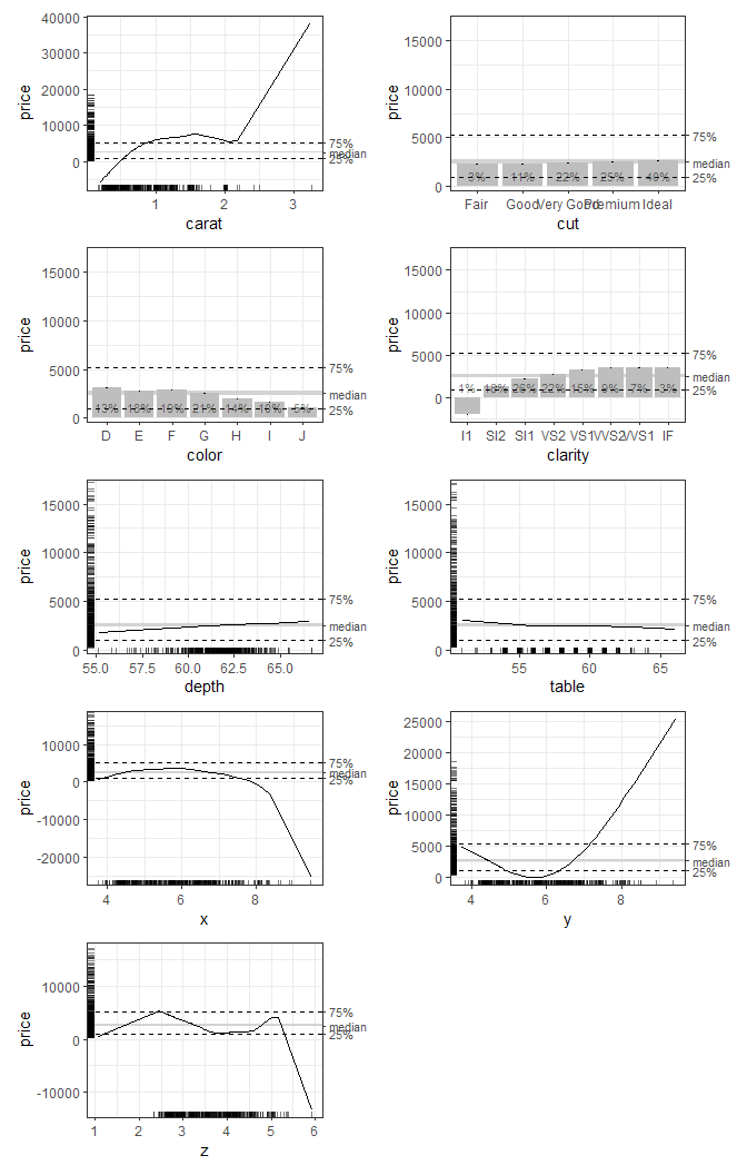
For an explanation of these basic features, see the introductory vignette.
The statistical functionality of the {ale} package is
rather slow because it typically involves 100 bootstrap iterations and
sometimes a 1,000 random simulations. Even though most functions in the
package implement parallel processing by default, such procedures still
take some time. So, this statistical demonstration gives you
downloadable objects for a rapid demonstration.
First, we need to create a p-value distribution object so that the ALE statistics can be properly distinguished from random effects.
# Create p_value distribution object
p_dist_gam_diamonds_readme <- retrieve_rds(
  # For speed, load a pre-created object by default.
  c(serialized_objects_site, 'p_dist_gam_diamonds_readme.0.5.2.rds'),
  {
    # Rather slow because it retrains the model 100 times.
    # To run the code yourself, execute this code block directly.
    ALEpDist(
      gam_diamonds, diamonds,
      # Normally should be default 1000, but just 100 for a quicker demo.
      rand_it = 100
    )
  }
)
# saveRDS(p_dist_gam_diamonds_readme, file.choose())
Now we can create bootstrapped ALE data and see some of the differences in the plots of bootstrapped ALE with p-values:
# Create ALE data with p-values

ale_gam_diamonds_stats_readme <- retrieve_rds(
  # For speed, load a pre-created object by default.
  c(serialized_objects_site, 'ale_gam_diamonds_stats_readme.0.5.2.rds'),
  {
    # To run the code yourself, execute this code block directly.
    ALE(
      gam_diamonds,
      # generate ALE for all 1D variables and the carat:clarity 2D interaction
      x_cols = list(d1 = TRUE, d2 = 'carat:clarity'),
      data = diamonds,
      p_values = p_dist_gam_diamonds_readme,
      # Usually at least 100 bootstrap iterations, but just 10 here for a faster demo
      boot_it = 10
    )
  }
)
# saveRDS(ale_gam_diamonds_stats_readme, file.choose())

# Create an ALEPlots object for fine-tuned plotting
ale_plots <- plot(ale_gam_diamonds_stats_readme)

# Plot 1D ALE plots
ale_plots |>
  # Only select 1D ALE plots.
  # Use subset() instead of get() to keep the special ALEPlots object
  # plot and print functionality.
  subset(list(d1 = TRUE)) |>
  print(ncol = 2)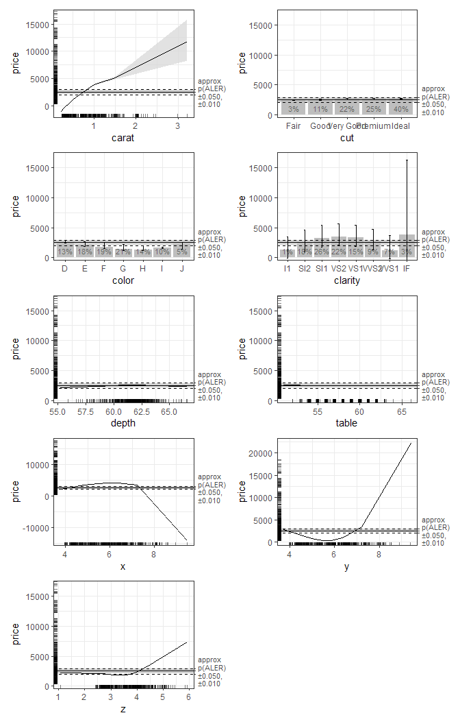
# Plot a selected 2D plot
ale_plots |>
  # get() retrieves a specific desired plot
get('carat:clarity') 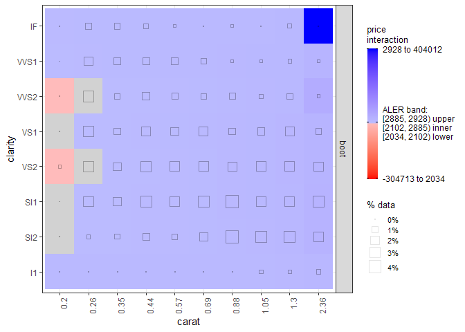
For a detailed explanation of how to interpret these plots, see the vignette on ALE-based statistics for statistical inference and effect sizes.
If you find a bug, please report it on GitHub. Be sure to
always include a minimal reproducible example for your usage requests.
If you cannot include your own dataset in the question, then use one of
the built-in datasets to frame your help request: var_cars
or census. You may also use ggplot2::diamonds
for a larger sample.
If you find this package useful, I would appreciate it if you would cite the appropriate sources as follows, depending on what aspects you use.
Apley, Daniel W., and Jingyu Zhu (2020). “Visualizing the effects of predictor variables in black box supervised learning models.” Journal of the Royal Statistical Society Series B: Statistical Methodology 82, no. 4: 1059-1086.
Okoli, Chitu (2023). “Statistical inference using machine learning and classical techniques based on accumulated local effects (ALE).” arXiv preprint arXiv:2310.09877.
Okoli, Chitu (2024). “Model-Agnostic Interpretability: Effect Size Measures from Accumulated Local Effects (ALE)”. INFORMS Workshop on Data Science 2024. Seattle
ale package (the software itself)Okoli, Chitu ([year of package version used]). “ale: Interpretable Machine Learning and Statistical Inference with Accumulated Local Effects (ALE)”. R software package version [enter version number]. https://CRAN.R-project.org/package=ale.