

![]()
![]()
aiRly is an unofficial R wrapper for Airly, platform which mission is to monitor and inform millions of people about the current state of air quality.
You can install current development version of aiRly from GitHub with:
devtools::install_github("piotrekjanus/aiRly")First, you should start with setting your Airly developer account at Airly developer. After you receive key, we can check air condition!
This is a basic example of package usage.
Let’s find out if there are any near stations somewhere in Krakow,
Poland. We will look for stations in a range of 20 km. We set
max_results to -1 in order to get all stations in the
neighborhood.
library(aiRly)

api_key <- Sys.getenv("api_key")
aiRly::set_apikey(api_key)

stations <- get_nearest_installations(50.11670, 19.91429, max_distance = 20, max_results = -1)
Let’s filter only for Airly stations and choose those which are located at the highest and lowest point a.s.l.
minmax_station <- stations %>%
                    filter(is_airly) %>%
                    summarize(min_elevation_id = id[which.min(elevation)],
                              max_elevation_id = id[which.max(elevation)])

h_station <- get_installation_measurements(minmax_station$max_elevation_id)
l_station <- get_installation_measurements(minmax_station$min_elevation_id)
Ok, we have just received information about current
state, last 24h history and forecasts for next
day for both installations.
Let’s make some visualizations
library(ggplot2)
library(gridExtra)

g1 <- ggplot() +
        geom_col(h_station$history, mapping = aes(x=time$from, y = measure$PM25, fill="High"),  alpha = 0.5) +
        geom_col(l_station$history, mapping = aes(x=time$from, y = measure$PM25, fill="Low"), alpha = 0.6) +
        scale_fill_manual(values=c("#40798C", "#CFD7C7")) +
        theme_minimal() +
        xlab("time") +
        ylab("PM25") +
        ggtitle("History") +
        theme(panel.grid.major.x = element_blank(),
              panel.grid.minor.x = element_blank(),
              plot.title = element_text(hjust=0.5),
              legend.position="top") +
        labs(fill="Installation")

g2 <- ggplot() +
        geom_col(h_station$forecast, mapping = aes(x=time$from, y = measure$PM25, fill="High"),  alpha = 0.5) +
        geom_col(l_station$forecast, mapping = aes(x=time$from, y = measure$PM25, fill="Low"), alpha = 0.6) +
        scale_fill_manual(values=c("#40798C", "#CFD7C7")) +
        theme_minimal() +
        xlab("time") +
        ylab("PM25") +
        ggtitle("Forecast") +
        theme(panel.grid.major.x = element_blank(),
              panel.grid.minor.x = element_blank(),
              plot.title = element_text(hjust=0.5),
              legend.position="top") +
        labs(fill="Installation")

grid.arrange(g1, g2, ncol = 2, nrow = 1)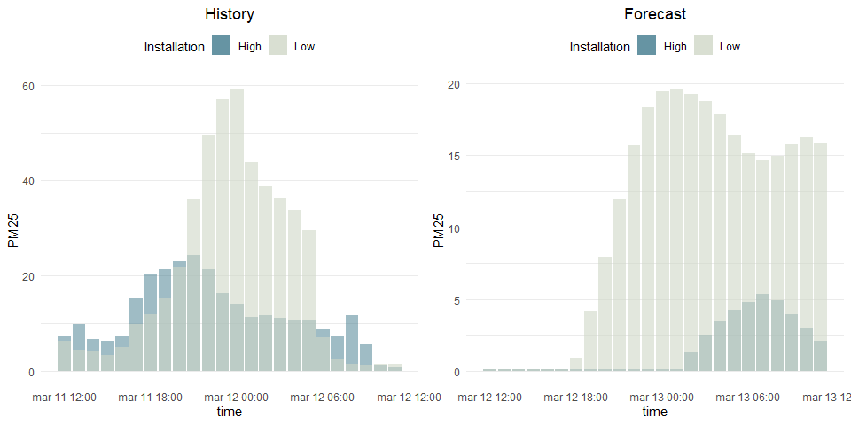
We can see that most of the time, air quality is worse (and will be)
in lower part of Krakow. Ok, but are those sensors readings indicating
high pollution? We can check it using get_indexes function,
which fill translate values of AIRLY_CAQI
variable
indexes <- get_indexes()
airly_caqi <- indexes %>% filter(name == "AIRLY_CAQI")
airly_caqi[is.na(airly_caqi)] <- Inf

history_high <- h_station$history
history_high$status <- unlist(lapply(history_high$index$AIRLY_CAQI,
                        function(x) airly_caqi[x >= airly_caqi$minValue &
                                               x <= airly_caqi$maxValue, "description"]))

history_low <- l_station$history
history_low$status <- unlist(lapply(history_low$index$AIRLY_CAQI,
                        function(x) airly_caqi[x >= airly_caqi$minValue &
                                               x <= airly_caqi$maxValue, "description"]))

ggplot() +
  geom_rect(history_high, mapping = aes(xmin=time$from, xmax = time$to,
                                        ymin=0, ymax=.1, fill = status)) +
  geom_rect(history_low, mapping = aes(xmin=time$from, xmax = time$to,
                                       ymin=0.2, ymax=.3, fill = status))+
  scale_fill_manual(values = c("Very Low" = "#6BC926",
                               "Low"    = "#D1CF1E",
                               "Medium" = "#EFBB0F",
                               "High"   = "#EF7120",
                               "Very High" ="#EF2A36",
                               "Extreme" = "#B00057",
                               "Airmageddon!" = "#770078")) +
  annotate("text", x = min(history_high$time$from), y = 0.25, label = "High a.s.l") +
  annotate("text", x = min(history_low$time$from), y = 0.05, label = "Low a.s.l") +
  theme_minimal() +
  theme(panel.grid = element_blank(),
        axis.text.y = element_blank()) +
  ylab("") +xlab("")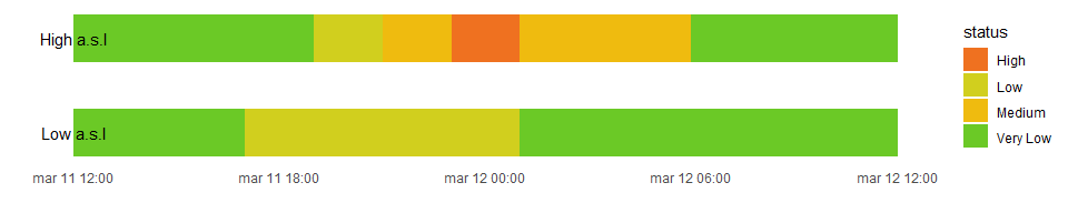
After we made few requests, we would like to check how many we have
left. For that purpose, simply use remaining_requests
rem_req <- remaining_requests()
cat("Available requests \n", rem_req$remaining, "/", rem_req$limit)
#> Available requests
#>  79 / 100