
![]()
![]()
The goal of affinity is to provide the basic tools used for raster grid georeferencing. This includes:
The main use at the moment is the ability to get a geotransform from an extent and dimension, this makes it easy to drive GDAL functions and to compare with the RasterIO logic in the sf package raster reader.
The main functions for georeferencing are affinething()
to collect drawn points interactively from an un-mapped raster image and
domath() to calculate the extent of the raster in
geographic terms and assignproj() to apply a map projection
inline. There are some other experimental functions to write GDAL VRT
gdalvrt() and to store some known cases for unmapped image
sources.
The basic tools still rely on the raster package.
You can install the dev version of affinity from GitHub with:
devtools::install_github("hypertidy/affinity")This examples takes an an un-mapped raster and georefences it by defining some control points for a simple (offset and scale) affine transformation.
Generally, we want diagonal points, so I tend to think “southwest” and “northeast”, it doesn’t really matter where they are as long as there’s some pixels between them in both directions. Monterey Bay is very recognizable so I read off some long-lat control points using mapview.
library(affinity)
data("montereybay", package = "rayshader")


library(raster)
#> Loading required package: sp
## we know that rayshader works transpose
r <- t(raster(montereybay))

prj <- "+proj=longlat +datum=WGS84"
## the north tip of Pacific Grove
sw <- c(-121.93348, 36.63674)
## the inlet at Moss Landing
ne <- c(-121.78825, 36.80592)
#mapview::mapview(c(sw[1], ne[1]), c(sw[2], ne[2]), crs = prj)
We can obtain raw (graphics) coordinates of those locations from our
image, by plotting it and clicking twice with
affinething().
Note the order, the first point is “sw” and the second is “ne” - the order is not important but it must match.
## mask the raster so we can see easily where we need to click
xy <- affinething(r > 0)
In this example the points are
xy <- structure(c(0.65805655219227, 0.858931100128933, 0.367586425626388,
0.589597209007295), .Dim = c(2L, 2L), .Dimnames = list(NULL,
    c("x", "y")))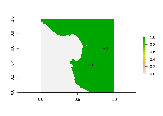
Now we have everything we need to re-map our raster! We don’t need to project our points as the known locations are in the same coordinate system as the source data. (In other situations we might georeference using a graticule on a projected map.)
mapped <- assignproj(setExtent(r, domath(rbind(sw, ne), xy, r, proj = NULL)), prj)

m <- rnaturalearth::ne_countries(country = "United States of America", scale = 10)
plot(mapped, col = viridis::viridis(30))
plot(m, add = TRUE)
contour(mapped, levels = -10, lty = 2, add = TRUE)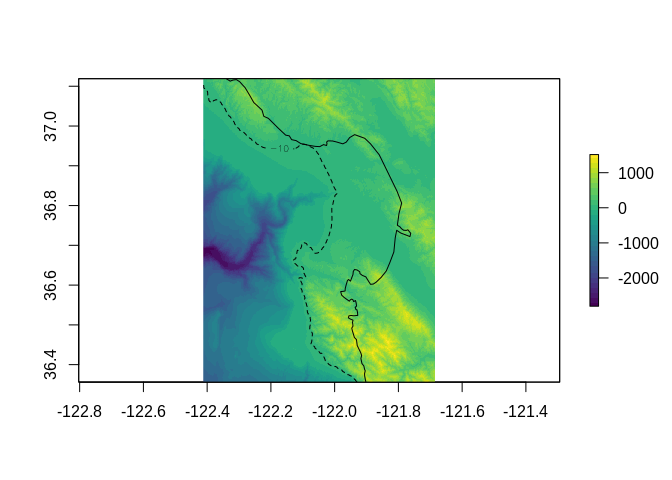
#mv <- mapview::mapview(mapped)Please note that the ‘affinity’ project is released with a Contributor Code of Conduct. By contributing to this project, you agree to abide by its terms.