
![]()

![]()
The adaptr package simulates adaptive (multi-arm,
multi-stage) clinical trials using adaptive stopping, adaptive arm
dropping and/or response-adaptive randomisation.
The package has been developed as part of the INCEPT (Intensive Care Platform Trial) project, primarily supported by a grant from Sygeforsikringen “danmark”.
Examples:
adaptr to assess the
performance of adaptive clinical trials according to different
follow-up/data collection lags.adaptr to assess the
performance of adaptive clinical trials according to different sceptical
priors.adaptr, see INCEPT and EMPRESS.The easiest way is to install from CRAN directly:
install.packages("adaptr")Alternatively, you can install the development version from GitHub - this requires the remotes-package installed. The development version may contain additional features not yet available in the CRAN version, but may not be stable or fully documented:
# install.packages("remotes")
remotes::install_github("INCEPTdk/adaptr@dev")The central functionality of adaptr and the typical
workflow is illustrated here.
First, the package is loaded and a cluster of parallel workers is
initiated by the setup_cluster() function to facilitate
parallel computing:
library(adaptr)
#> Loading 'adaptr' package v1.5.0.
#> For instructions, type 'help("adaptr")'
#> or see https://inceptdk.github.io/adaptr/.

setup_cluster(2)Setup a trial specification (defining the trial design and scenario)
using the general setup_trial() function, or one of the
special case variants using default priors
setup_trial_binom() (for binary, binomially distributed
outcomes; used in this example) or setup_trial_norm() (for
continuous, normally distributed outcomes).
# Setup a trial using a binary, binomially distributed, undesirable outcome
binom_trial <- setup_trial_binom(
  arms = c("Arm A", "Arm B", "Arm C"),
  # Scenario with identical outcomes in all arms
  true_ys = c(0.25, 0.25, 0.25),
  # Response-adaptive randomisation with minimum 20% allocation in all arms
  min_probs = rep(0.20, 3),
  # Number of participants with data available at each analysis
  data_looks = seq(from = 300, to = 2000, by = 100),
  # Number of participants randomised at each analysis (higher than the numbers
  # with data, except at last look, due to follow-up/data collection lag)
  randomised_at_looks = c(seq(from = 400, to = 2000, by = 100), 2000),
  # Stopping rules for inferiority/superiority not explicitly defined
  # Stop for equivalence at > 90% probability of differences < 5 %-points
  equivalence_prob = 0.9,
  equivalence_diff = 0.05
)

# Print trial specification
print(binom_trial, prob_digits = 3)
#> Trial specification: generic binomially distributed outcome trial
#> * Undesirable outcome
#> * No common control arm
#> * Best arms: Arm A and Arm B and Arm C
#>
#> Arms, true outcomes, starting allocation probabilities
#> and allocation probability limits (fixed/min/max_probs not rescaled):
#>   arms true_ys start_probs fixed_probs min_probs max_probs
#>  Arm A    0.25       0.333          NA       0.2        NA
#>  Arm B    0.25       0.333          NA       0.2        NA
#>  Arm C    0.25       0.333          NA       0.2        NA
#>
#> Maximum sample size: 2000
#> Maximum number of data looks: 18
#> Planned data looks after:  300, 400, 500, 600, 700, 800, 900, 1000, 1100, 1200, 1300, 1400, 1500, 1600, 1700, 1800, 1900, 2000 participants have reached follow-up
#> Number of participants randomised at each look:  400, 500, 600, 700, 800, 900, 1000, 1100, 1200, 1300, 1400, 1500, 1600, 1700, 1800, 1900, 2000, 2000
#>
#> Superiority threshold: 0.99 (all analyses)
#> Inferiority threshold: 0.01 (all analyses)
#> Equivalence threshold: 0.9 (all analyses) (no common control)
#> Absolute equivalence difference: 0.05
#> No futility threshold (not relevant - no common control)
#> Adaptation rule probability thresholds not rescaled when arms are dropped
#> Soften power for all analyses: 1 (no softening)In the example trial specification, there are no true between-arm
differences, and stopping rules for inferiority and superiority are not
explicitly defined. This is intentional, as these stopping rules will be
calibrated to obtain a desired probability of stopping for superiority
in the scenario with no between-arm differences (corresponding to the
Bayesian type 1 error rate). Trial specifications do not necessarily
have to be calibrated, and simulations can be run directly using the
run_trials() function covered below (or
run_trial() for a single simulation).
Calibration of a trial specification is done using the
calibrate_trial() function, which defaults to calibrate
constant, symmetrical stopping rules for inferiority and superiority
(expecting a trial specification with identical outcomes in each arm),
but can be used to calibrate any parameter in a trial specification
towards any performance metric.
# Calibrate the trial specification
calibrated_binom_trial <- calibrate_trial(
  trial_spec = binom_trial,
  n_rep = 1000, # 1000 simulations for each step (more generally recommended)
  base_seed = 4131, # Base random seed (for reproducible results)
  target = 0.05, # Target value for calibrated metric (default value)
  search_range = c(0.9, 1), # Search range for superiority stopping threshold
  tol = 0.01, # Tolerance range
  dir = -1 # Tolerance range only applies below target
)

# Print result (to check if calibration is successful)
calibrated_binom_trial
#> Trial calibration:
#> * Result: calibration successful
#> * Best x: 0.9814318
#> * Best y: 0.048
#>
#> Central settings:
#> * Target: 0.05
#> * Tolerance: 0.01 (at or below target, range: 0.04 to 0.05)
#> * Search range: 0.9 to 1
#> * Gaussian process controls:
#> * - resolution: 5000
#> * - kappa: 0.5
#> * - pow: 1.95
#> * - lengthscale: 1 (constant)
#> * - x scaled: yes
#> * Noisy: no
#> * Narrowing: yes
#>
#> Calibration/simulation details:
#> * Total evaluations: 7 (previous + grid + iterations)
#> * Repetitions: 1000
#> * Calibration time: 3.87 mins
#> * Base random seed: 4131
#>
#> See 'help("calibrate_trial")' for details.
The calibration is successful - the calibrated, constant stopping
threshold for superiority is printed with the results (0.9814318) and
can be extracted using calibrated_binom_trial$best_x. Using
the default calibration functionality, the calibrated, constant stopping
threshold for inferiority is symmetrical, i.e.,
1 - stopping threshold for superiority (0.0185682). The
calibrated trial specification may be extracted using
calibrated_binom_trial$best_trial_spec and, if printed,
will also include the calibrated stopping thresholds.
Calibration results may be saved (and reloaded) by using the
path argument, to avoid unnecessary repeated
simulations.
The results of the simulations using the calibrated trial
specification conducted during the calibration procedure may be
extracted using calibrated_binom_trial$best_sims. These
results can be summarised with several functions. Most of these
functions support different ‘selection strategies’ for simulations not
ending with superiority, i.e., performance metrics can be calculated
assuming different arms would be used in clinical practice if no arm is
ultimately superior.
The check_performance() function summarises performance
metrics in a tidy data.frame, with uncertainty measures
(bootstrapped confidence intervals) if requested. Here, performance
metrics are calculated considering the ‘best’ arm (i.e., the one with
the highest probability of being overall best) selected in simulations
not ending with superiority:
# Calculate performance metrics with uncertainty measures
binom_trial_performance <- check_performance(
  calibrated_binom_trial$best_sims,
  select_strategy = "best",
  uncertainty = TRUE, # Calculate uncertainty measures
  n_boot = 1000, # 1000 bootstrap samples (more typically recommended)
  ci_width = 0.95, # 95% confidence intervals (default)
  boot_seed = "base" # Use same random seed for bootstrapping as for simulations
)

# Print results
print(binom_trial_performance, digits = 2)
#>                   metric     est err_sd err_mad   lo_ci   hi_ci
#> 1           n_summarised 1000.00   0.00    0.00 1000.00 1000.00
#> 2              size_mean 1749.60  11.36   10.97 1727.20 1772.10
#> 3                size_sd  373.74   9.64    9.74  355.15  392.58
#> 4            size_median 2000.00   0.00    0.00 2000.00 2000.00
#> 5               size_p25 1400.00  52.43    0.00 1400.00 1500.00
#> 6               size_p75 2000.00   0.00    0.00 2000.00 2000.00
#> 7                size_p0  400.00     NA      NA      NA      NA
#> 8              size_p100 2000.00     NA      NA      NA      NA
#> 9            sum_ys_mean  438.69   2.95    2.85  432.74  444.66
#> 10             sum_ys_sd   96.20   2.42    2.37   91.28  100.79
#> 11         sum_ys_median  486.00   1.98    2.97  483.00  490.00
#> 12            sum_ys_p25  364.75  10.95    9.64  352.00  395.00
#> 13            sum_ys_p75  506.00   1.15    1.48  504.00  508.00
#> 14             sum_ys_p0   88.00     NA      NA      NA      NA
#> 15           sum_ys_p100  565.00     NA      NA      NA      NA
#> 16         ratio_ys_mean    0.25   0.00    0.00    0.25    0.25
#> 17           ratio_ys_sd    0.01   0.00    0.00    0.01    0.01
#> 18       ratio_ys_median    0.25   0.00    0.00    0.25    0.25
#> 19          ratio_ys_p25    0.24   0.00    0.00    0.24    0.24
#> 20          ratio_ys_p75    0.26   0.00    0.00    0.26    0.26
#> 21           ratio_ys_p0    0.20     NA      NA      NA      NA
#> 22         ratio_ys_p100    0.30     NA      NA      NA      NA
#> 23       prob_conclusive    0.43   0.02    0.01    0.40    0.46
#> 24         prob_superior    0.05   0.01    0.01    0.04    0.06
#> 25      prob_equivalence    0.38   0.02    0.01    0.35    0.41
#> 26         prob_futility    0.00   0.00    0.00    0.00    0.00
#> 27              prob_max    0.57   0.02    0.01    0.54    0.60
#> 28 prob_select_arm_Arm A    0.32   0.02    0.01    0.29    0.35
#> 29 prob_select_arm_Arm B    0.31   0.01    0.01    0.28    0.34
#> 30 prob_select_arm_Arm C    0.37   0.02    0.02    0.34    0.40
#> 31      prob_select_none    0.00   0.00    0.00    0.00    0.00
#> 32                  rmse    0.02   0.00    0.00    0.02    0.02
#> 33               rmse_te      NA     NA      NA      NA      NA
#> 34                   mae    0.01   0.00    0.00    0.01    0.01
#> 35                mae_te      NA     NA      NA      NA      NA
#> 36                   idp      NA     NA      NA      NA      NA
Similar results in list format (without uncertainty
measures) can be obtained using the summary() method, which
comes with a print() method providing formatted
results:
binom_trial_summary <- summary(
  calibrated_binom_trial$best_sims,
  select_strategy = "best"
)

print(binom_trial_summary)
#> Multiple simulation results: generic binomially distributed outcome trial
#> * Undesirable outcome
#> * Number of simulations: 1000
#> * Number of simulations summarised: 1000 (all trials)
#> * No common control arm
#> * Selection strategy: best remaining available
#> * Treatment effect compared to: no comparison
#>
#> Performance metrics (using posterior estimates from final analysis [all participants]):
#> * Sample sizes: mean 1749.6 (SD: 373.7) | median 2000.0 (IQR: 1400.0 to 2000.0) [range: 400.0 to 2000.0]
#> * Total summarised outcomes: mean 438.7 (SD: 96.2) | median 486.0 (IQR: 364.8 to 506.0) [range: 88.0 to 565.0]
#> * Total summarised outcome rates: mean 0.251 (SD: 0.011) | median 0.250 (IQR: 0.244 to 0.258) [range: 0.198 to 0.295]
#> * Conclusive: 42.9%
#> * Superiority: 4.8%
#> * Equivalence: 38.1%
#> * Futility: 0.0% [not assessed]
#> * Inconclusive at max sample size: 57.1%
#> * Selection probabilities: Arm A: 31.8% | Arm B: 31.0% | Arm C: 37.2% | None: 0.0%
#> * RMSE / MAE: 0.01730 / 0.01102
#> * RMSE / MAE treatment effect: not estimated / not estimated
#> * Ideal design percentage: not estimable
#>
#> Simulation details:
#> * Simulation time: 35.5 secs
#> * Base random seed: 4131
#> * Credible interval width: 95%
#> * Number of posterior draws: 5000
#> * Estimation method: posterior medians with MAD-SDs
Individual simulation results may be extracted in a tidy
data.frame using extract_results().
Finally, the probabilities of different remaining arms and their
statuses (with uncertainty) at the last adaptive analysis can be
summarised using the check_remaining_arms() function.
Several visualisation functions are included (all are optional, and
all require the ggplot2 package installed).
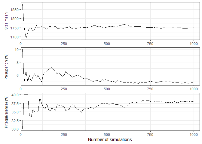
Convergence and stability of one or more performance metrics may be
visually assessed using plot_convergence() function:
plot_convergence(
  calibrated_binom_trial$best_sims,
  metrics = c("size mean", "prob_superior", "prob_equivalence"),
  # select_strategy can be specified, but does not affect the chosen metrics
)
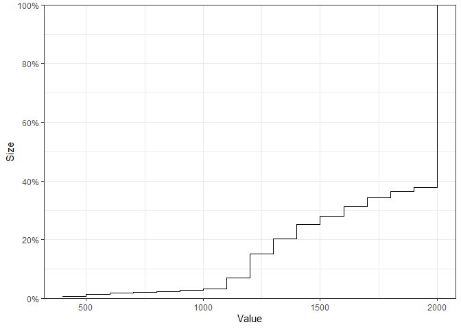
The empirical cumulative distribution functions for continuous performance metrics may also be visualised:
plot_metrics_ecdf(
  calibrated_binom_trial$best_sims,
  metrics = "size"
)
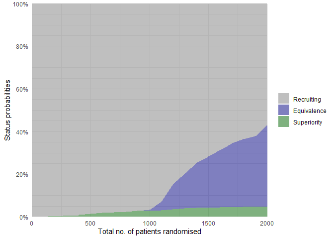
The status probabilities for the overall trial (or for specific arms)
according to trial progress can be visualised using the
plot_status() function:
# Overall trial status probabilities
plot_status(
  calibrated_binom_trial$best_sims,
  x_value = "total n" # Total number of randomised participants at X-axis
)
Finally, various metrics may be summarised over the progress of one
or multiple trial simulations using the plot_history()
function, which requires non-sparse results (the sparse
argument must be FALSE in calibrate_trials(),
run_trials(), or run_trial(), leading to
additional results being saved).
The calibrated stopping thresholds (calibrated in a scenario with no between-arm differences) may be used to run simulations with the same overall trial specification, but according to a different scenario (i.e., with between-arm differences present) to assess performance metrics (including the Bayesian analogue of power).
First, a new trial specification is setup using the same settings as before, except for between-arm differences and the calibrated stopping thresholds:
binom_trial_calib_diff <- setup_trial_binom(
  arms = c("Arm A", "Arm B", "Arm C"),
  true_ys = c(0.25, 0.20, 0.30), # Different outcomes in the arms
  min_probs = rep(0.20, 3),
  data_looks = seq(from = 300, to = 2000, by = 100),
  randomised_at_looks = c(seq(from = 400, to = 2000, by = 100), 2000),
  # Stopping rules for inferiority/superiority explicitly defined
  # using the calibration results
  inferiority = 1 - calibrated_binom_trial$best_x,
  superiority = calibrated_binom_trial$best_x,
  equivalence_prob = 0.9,
  equivalence_diff = 0.05
)
Simulations using the trial specification with calibrated stopping
thresholds and differences present can then be conducted using the
run_trials() function and performance metrics calculated as
above:
binom_trial_diff_sims <- run_trials(
  binom_trial_calib_diff,
  n_rep = 1000, # 1000 simulations (more generally recommended)
  base_seed = 1234 # Reproducible results
)

check_performance(
  binom_trial_diff_sims,
  select_strategy = "best",
  uncertainty = TRUE,
  n_boot = 1000, # 1000 bootstrap samples (more typically recommended)
  ci_width = 0.95,
  boot_seed = "base"
)
#>                   metric      est err_sd err_mad    lo_ci    hi_ci
#> 1           n_summarised 1000.000  0.000   0.000 1000.000 1000.000
#> 2              size_mean 1242.300 16.620  16.976 1209.895 1273.025
#> 3                size_sd  531.190  7.251   7.604  516.617  544.091
#> 4            size_median 1200.000 22.220   0.000 1200.000 1300.000
#> 5               size_p25  800.000 36.095   0.000  700.000  800.000
#> 6               size_p75 1700.000 42.453   0.000 1700.000 1800.000
#> 7                size_p0  400.000     NA      NA       NA       NA
#> 8              size_p100 2000.000     NA      NA       NA       NA
#> 9            sum_ys_mean  284.999  3.695   3.726  277.724  291.991
#> 10             sum_ys_sd  117.265  1.701   1.732  113.765  120.311
#> 11         sum_ys_median  279.000  5.268   4.448  269.500  289.512
#> 12            sum_ys_p25  186.000  6.682   7.413  174.000  197.019
#> 13            sum_ys_p75  390.000  7.633   7.413  374.000  402.250
#> 14             sum_ys_p0   81.000     NA      NA       NA       NA
#> 15           sum_ys_p100  519.000     NA      NA       NA       NA
#> 16         ratio_ys_mean    0.232  0.000   0.001    0.231    0.233
#> 17           ratio_ys_sd    0.016  0.000   0.000    0.015    0.017
#> 18       ratio_ys_median    0.230  0.001   0.000    0.230    0.232
#> 19          ratio_ys_p25    0.221  0.000   0.000    0.220    0.222
#> 20          ratio_ys_p75    0.242  0.001   0.001    0.240    0.243
#> 21           ratio_ys_p0    0.195     NA      NA       NA       NA
#> 22         ratio_ys_p100    0.298     NA      NA       NA       NA
#> 23       prob_conclusive    0.877  0.011   0.010    0.857    0.898
#> 24         prob_superior    0.731  0.014   0.015    0.706    0.759
#> 25      prob_equivalence    0.146  0.011   0.011    0.125    0.167
#> 26         prob_futility    0.000  0.000   0.000    0.000    0.000
#> 27              prob_max    0.123  0.011   0.010    0.102    0.143
#> 28 prob_select_arm_Arm A    0.038  0.006   0.006    0.026    0.049
#> 29 prob_select_arm_Arm B    0.962  0.006   0.006    0.951    0.974
#> 30 prob_select_arm_Arm C    0.000  0.000   0.000    0.000    0.000
#> 31      prob_select_none    0.000  0.000   0.000    0.000    0.000
#> 32                  rmse    0.020  0.001   0.001    0.019    0.022
#> 33               rmse_te       NA     NA      NA       NA       NA
#> 34                   mae    0.011  0.000   0.000    0.010    0.012
#> 35                mae_te       NA     NA      NA       NA       NA
#> 36                   idp   98.100  0.306   0.297   97.549   98.700
Again, simulations may be saved and reloaded using the
path argument.
Similarly, overall trial statuses for the scenario with differences can be visualised:
plot_status(binom_trial_diff_sims, x_value = "total n")
We use the GitHub issue tracker for all bug/issue reports and proposals for enhancements.
We welcome contributions directly to the code to improve performance as well as new functionality. For the latter, please first explain and motivate it in an issue.
Changes to the code base should follow these steps:
NEWS.md file to see the formatting)dev branch of adaptrIf you use the package, please consider citing it:
citation(package = "adaptr")
#> To cite package 'adaptr' in publications use:
#>
#>   Granholm A, Jensen AKG, Lange T, Kaas-Hansen BS (2022). adaptr: an R
#>   package for simulating and comparing adaptive clinical trials.
#>   Journal of Open Source Software, 7(72), 4284. URL
#>   https://doi.org/10.21105/joss.04284.
#>
#>   Granholm A, Jensen AKG, Lange T, Perner A, Møller MH, Kaas-Hansen BS
#>   (2025). Designing and Evaluating Bayesian Advanced Adaptive
#>   Randomised Clinical Trials: A Practical Guide. Pharmaceutical
#>   Statistics, 24(6), e70042. URL https://doi.org/10.1002/pst.70042.
#>
#> To see these entries in BibTeX format, use 'print(<citation>,
#> bibtex=TRUE)', 'toBibtex(.)', or set
#> 'options(citation.bibtex.max=999)'.