

This package allows you to visualize the number of downloads for an specific package in the CRAN repository.
The user can specify different ways to display the information: in a classic (static) plot, an interactive representation, and/or a combined figure comparing multiple packages.
The user can specify the range of dates to be processed, however the main function of the package will run a couple of checks and adjustments on these:
if no dates are specified it will assume the current date as the end of the period and a year before as the starting date, ie. a period of a year since today;
given a range of dates, it will reset the range to the first reported download within the specified dates, so that dates previous to any reported download from the CRAN logs are not shown, in this way the package can generate a cleaner and more meaningful visualization.
In order to show a closer trend to the time series data of downloads, the package will also display moving avera ges and moving intervals of confidence. The confidence interval will be shaded in the main plot.
Both features can be turned off, using the corresponding flags in the
options: "noMovAvg" and "noConfBands".
The moving estimators (average and confidence intervarls) are comoputed using a default of 10 windows to be considered over the indicated period of time, i.e. in a given period of time the algorithm will select 10 windows resulting in an effective size for the moving window of the time range divived by 10. The confidence interval is determined using the “moving” standard deviation, ie. the standard deviation computed on the moving window. The upper limit of the confidence band is determined by +half standard deviation and the lower band by -half standard deviation in the corresponding window.
Visualize.CRAN.Downloads utilizes the cranlogs package
for accessing the data of the downloads and the plotly
package for generating interactive visualizations. The basic (static)
plots are generated employing R basic capabilities. The basic plots are
saved in the current directory in a PDF file named
“DWNLDS_packageName.pdf”, where
‘packageName’ is the actual name of the
package analyzed. The interactive plots are saved in the current
directory in an HTML file named
“Interactive_DWNLDS_packageName.html”, where
‘packageName’ is the actual name of the
package analyzed.
The following are the main functions that can be used in the “Visualize.CRAN.Downloads” package:
| Function | Description |
|---|---|
processPckg |
this is the main function that can be used specifying the package(s) name(s), as well as other options |
staticPlots |
this function will generate the static plots for a given package’s data |
interactivePlots |
this function will generate the interactive plots for a given package’s data |
comparison.Plt |
this function will generate a comparison plot among multiple packages |
With all these functions, it is possible to specify several packages at the same time, and indicate the type of outcome to be produced.
The processPckg function will generate by default the
static and interactive representations, this can be turned off by
indicating the "nostatic" and/or
"nointeractive" as options in the arguments of the main
function.
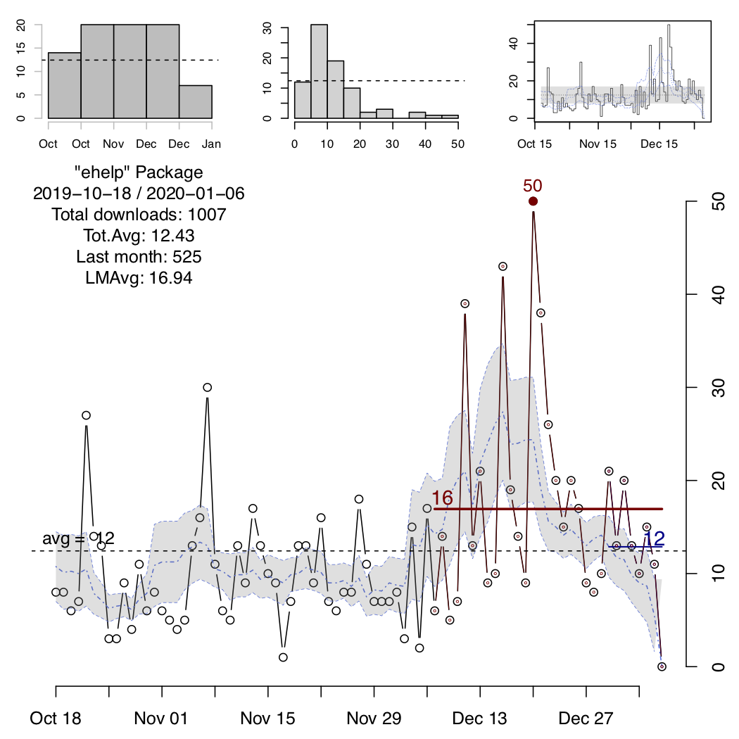
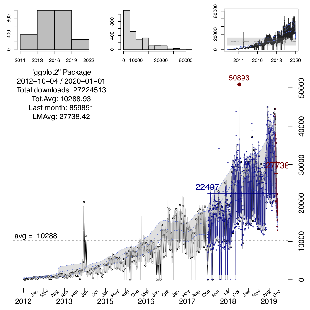
The static plot actually includes 4 different plots: a histogram of
downloads vs time, a histogram of number of downloads, a pulse plot and
a download vs time plot. The default style is to generate these 4 plots
in the same figure, but it can be switch to generate one plot per figure
by utilizing the "nocombined" option. In each of the plot a
dahsed line is added representing the total average over time. In the
“pulse” plot (third subplot), we added also a shaded region defined by
the total average plus/minus the total standard deviation. Additionally,
moving averages and moving standard deviations computations are
displayed in dotted and dased-dotted lines. The main plot also displays
the total average and the shaded region corresponds to the confidence
interval defined by the moving average plus/minus the moving standard
deviation computed using a window of 1/10 the length of the period of
time. The display of the moving estimators can be turned off, including
the "noMovAvg" flag; and the shaded regions can be avoided
using the "noConfBand" flag.
Two more “fixed” averages are presented in the main plot, indicating the average number of downloads for the package in the last two “units” of time, eg last month and last week, or last six-months and last month, etc. The absolute maximum number of downloads within the period of time, is also displayed as a filled dot and the actual value.
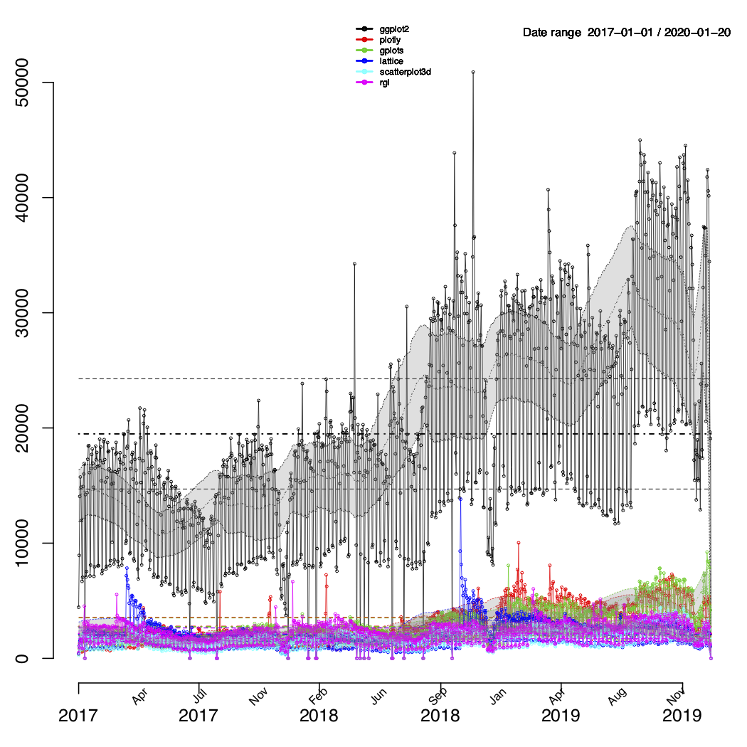
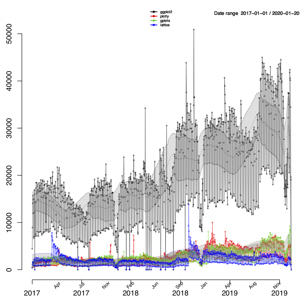
A comparison plot between multiple package should be explicity
requested using the "compare" option in the list of
arguments of the processPckg function.
For using this feature more than one package should be indicated!
The comparison plot will be saved into a PDF file named
“DWNLDS_packageNames.pdf”, where
packageNames is the combination of all the packages
indicated to process. When the "compare" option is
indicated, it will also check for the "nocombined" option
to either generate the comparison plot combining all packages in the
same plot or in separated ones, but always within the same file.
Similarly, the "noMovAvg" and "noConfBand"
flags can be used for turning off the moving averages indicators and
overall average ones.
Additionally, when the "compare" option is indicated the
processPckg function will return a nested list containing
in each element a list with the information of each the packages, ie.
date-downloads-package.name.
Interactive plots are generated using the plotly package
and combine two plots in one single html file.
The left plot will highlight the last month of data, and the plot on the right uses colour and symbols size to represent the respective downloads. The size of the symbols is rescaled with respect to the maximum number of downloads within the given time period, so it actuallty represents relative values.
   <p>A live example of this can be seen at
        <a href="https://mponce0.github.io/Visualize.CRAN.Downloads/">https://mponce0.github.io/Visualize.CRAN.Downloads/</a>
</p>opts argument of the
processPckg function| option | action |
|---|---|
"nostatic" |
disables static plots |
"nointeractive" |
disables interactive plots |
"nocombined" |
disables combination of static plots, ie. each plot will be a separated figure |
"noConfBand" |
disables the shading of “confidence bands (regions)” |
"noMovAvg" |
disables the display of “moving” estimators |
"compare" |
generates a plot comparing the downloads of multiple packages |
"noSummary" |
disables the output of the stats-time summaries presented per package |
In addition the processPckg function also takes the
following arguments:
| argument | description |
|---|---|
pckg.lst |
list of packages to process |
t0 |
initial date, begining of the time period, given in “YYYY-MM-DD” format |
t1 |
final date, ending of the time period, given in “YYYY-MM-DD” format |
opts |
a list of different options available for customizing the output |
device |
string to select the output format: ‘PDF’/‘PNG’/‘JPEG’ or ‘screen’ |
For using the “Visualize.CRAN.Downloads” package, first you will need
to install it. “Visualize.CRAN.Downloads” requires the
cranlogs and plotly packages, check to have
these already installed before installing
Visualize.CRAN.Downloads.
The stable version can be downloaded from the CRAN repository:
install.packages("Visualize.CRAN.Downloads")To obtain the development version you can get it from the github repository, i.e.
# need devtools for installing from the github repo
install.packages("devtools")

# install Visualize.CRAN.Downloads
devtools::install_github("mponce0/Visualize.CRAN.Downloads")
After having installed the “Visualize.CRAN.Downloads” package, you will need to load it into your R session or R script:
# load Visualize.CRAN.Downloads
library(Visualize.CRAN.Downloads)processPckg()# generates static and interactive plots for the "ehelp" package with default arguments
# default value for the static plot is PDF
processPckg("ehelp")
# specifying starting date in 2001-01-01, and send to the screen
processPckg(c("ehelp","plotly","ggplot"), "2001-01-01", device="SCREEN")
# request no static plot, ie. only interactive plot will be generated
processPckg(c("ehelp","plotly","ggplot"), "2001-01-01", opts="nostatic")
# process 3 packages, with only static plot, ie. no interactive nor comparison plot
# static plots will be genereated as PDF
processPckg(c("ehelp","plotly","ggplot"), "2001-01-01", opts=c("nointeractive","nocombined"))
# process 4 packages, with a given starting date and static and comparison plots
# output set to screen
pckg.data <- processPckg(c('ggplot2','plotly','gplots','lattice'), '2017-01-01',
opts=c('nointeractive','compare','noConfBand'), device='SCREEN')
# no interactive plot, only static plots for each package and comparison plot among all of them to be displayed in 'screen' only
pckg.data <- processPckg(c('plotly','gplots','lattice','scatterplot3d','rgl'), '2017-01-01',
opts=c('nointeractive','compare','noMovAvg','noConfBand'), device="SCREEN")staticPlots()# retrieve data
packageData <- retrievePckgData("ggplot")
# select 1st element of the list
totalDownloads <- packageData[[1]]
# call the plotting fn, with default value of device --> PDF
staticPlots(totalDownloads)
# set output to the screen
staticPlots(totalDownloads,combinePlts=TRUE, device='SCREEN')interactivePlots()# retrieve data and select first element of the list
packageXdownloads <- retrievePckgData("ggplot")[[1]]
# invoque the interacive plotting fn
interactivePlots(packageXdownloads)Employing the basic plotting functions from the
“Visualize.CRAN.Downloads” package, staticPlots(),
interactivePlots() and comparison.Plt(), it is
also possible to generate plots for packages from BioConductor. The data
must be downloaded separatedly, for instance, using the “bioC.logs”
(https://github.com/mponce0/bioC.logs) package:
# install bioC.logs from CRAN
install.packages("bioC.logs")

# load bioC.logs
library(bioC.logs)

# retrieve stats for BioConductor packages using the bioC.logs package
# Notice that the "CRAN" format is needed in the the bioC_downloads() fn
# Also that we are slicing the first (and only element) of the returned list
edgeR.logs <- bioC_downloads("edgeR", format="CRAN")[[1]]

# generate plots for the BioConductor package stats
staticPlots(edgeR.logs, combinePlts=TRUE, device="SCREEN")
interactivePlots(edgeR.logs)One useful application this package offers is the chance to
automatically generate figures reporting the statistics of your favorite
package. For such, you can create a cron job using the
following Rscript.
## queryScript.R

# load library
library(Visualize.CRAN.Downloads)

# query fav. package
# this will generate the PDF static and HTML interactive plot, with the default one-year time window
processPckg("ehelp", device="PDF")
Then your cron script would be something like,
## myCRONscript

0 5 * * * Rscript /home/username/scripts/queryScript.R
this would run the Rscript queryScript.R querying the
‘ehelp’ package every day at 5AM generating the static PDF and
interactive HTML figures.
For having this execute, you will only need to run the following command in the shell:
$ crontab /home/username/myCRONscriptAlternatively instead of calling the Rscript directly in your cron-job, you could execute a shell script that executes the Rscript first and then pushes the plots to your github repository. For instance,
## updateREPORTS.sh

# first call the Rscript to generate plots
Rscript /home/username/scripts/queryScript.R

# now add your files to your repo
# this assumes that you have set up your repo using your keys as credentials
git add /home/username/DWNLDS_favPckg.pdf
git add /home/username/DWNLDS_favPckg.pdf

# push the changes to the central github-repo
# this will make them accesible through your repo, basically updating them every day at 5AM
git push
The cron-job script would in this case look like:
## myCRONscript

0 5 * * * /home/username/scripts/updateREPORTS.sh> citation("Visualize.CRAN.Downloads")
To cite package ‘Visualize.CRAN.Downloads’ in publications use:
Marcelo Ponce (2020). Visualize.CRAN.Downloads: Visualize Downloads
from 'CRAN' Packages. R package version 1.0.
https://CRAN.R-project.org/package=Visualize.CRAN.Downloads
A BibTeX entry for LaTeX users is
@Manual{,
title = {Visualize.CRAN.Downloads: Visualize Downloads from 'CRAN' Packages},
author = {Marcelo Ponce},
year = {2020},
note = {R package version 1.0},
url = {https://CRAN.R-project.org/package=Visualize.CRAN.Downloads},
}
