{STMr} Package
{STMr} Package
![]()
Table of Contents
This is longer README file, so here is the TOC for easier jumping to topics
{STMr}{STMr} (short of Strength Training Manual
R-functions) package is created to help sports scientists and
strength coaches estimate strength profiles, create and visualize
(percent-based) progression tables and set and rep schemes. Originally
{STMr} package was created as an internal project/package
to help me in writing Strength
Training Manual Volume 3 book, but it soon became a project in
itself. {STMr} package is open-source package under MIT
License implemented in the R language.
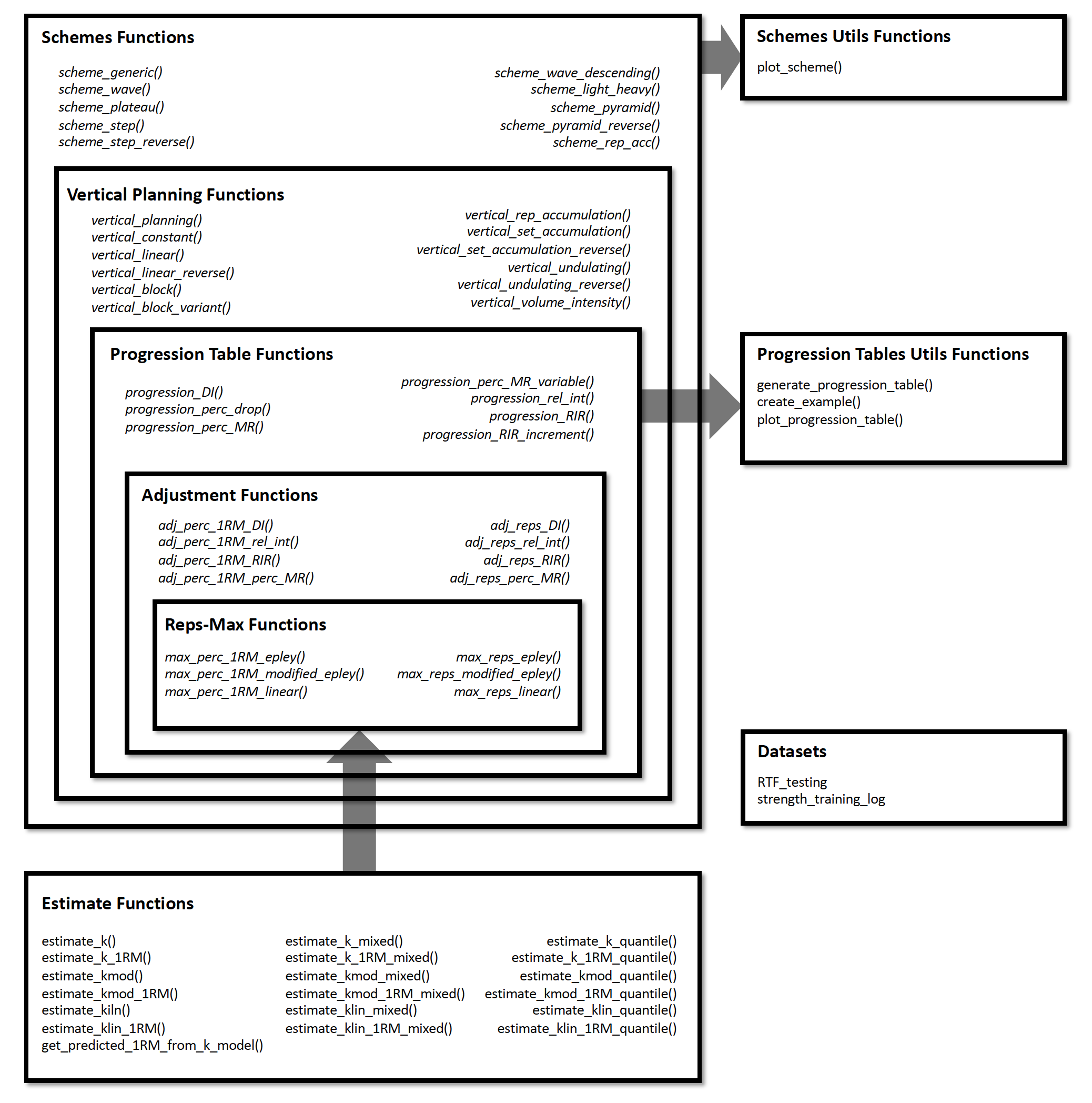
{STMr} package can be divided in the following
functional units:
max_)adj_)get_reps() and
get_perc_1RM() are implemented to combine Reps-Max models
as well as progression (adjustment) functions into easy to use
formatprogression_)vertical_)scheme_)release() function for molding multiple back-to-back
schemes (i.e., blocks or phases)generate_progression_table(),
plot_progression_table(), plot_scheme()
(deprecated as of {STMr} version 0.1.4. Please use S3
plot() method instead), and
create_example()strength_training_log and
RTF_testing)estimate_)Figure below depicts the relationship between {STMr}
package functional units:
I will walk you through each of these functional units to demonstrate
the simplicity, flexibility, usability, and power of the
{STMr} package. For more information regarding the logic
behind the {STMr} package please check the Load-Exertion
Tables And Their Use For Planning article series.
You can install the released version (once released) of
{STMr} from CRAN
with:
install.packages("STMr")And the development version from GitHub with:
# install.packages("devtools")
devtools::install_github("mladenjovanovic/STMr")
Once installed, you can load {STMr} package:
library(STMr)Reps-Max functions map the relationship between %1RM and maximum
number of repetitions (nRM, MNR, or reps-to-failure;
RTF). {STMr} package comes with three Reps-Max
models: (1) Epley’s, (2) Modified Epley’s, and (3) Linear/Brzycki’s.
Please refer to Load-Exertion
Tables And Their Use For Planning article series for more
information.
Reps-Max functions start with max_ and allow you to
either predict max %1RM from repetitions (start with
max_perc_1RM_), or to predict max repetitions (i.e., nRM)
from %1RM used (start with max_reps_). Each of Reps-Max
functions allow you to use different model parameter values. This is
very helpful when using individualized profiles to create set and rep
schemes (see Estimation section).
Let’s say I am interested in predicting max %1RM that can be used for doing 5 reps to failure. Here you can see how three different models can be used, together with providing custom parameter values:
# Predicting max %1RM to be used for target number of repetitions (to failure)

# ------------------------------------------
# Epley equation
max_perc_1RM_epley(5) # Default k=0.0333
#> [1] 0.857
max_perc_1RM_epley(5, k = 0.04)
#> [1] 0.833

# ------------------------------------------
# Modified Epley equation
max_perc_1RM_modified_epley(5) # Default kmod=0.0353
#> [1] 0.876
max_perc_1RM_modified_epley(5, kmod = 0.05)
#> [1] 0.833

# ------------------------------------------
# Linear/Brzycki equation
max_perc_1RM_linear(5) # Default klin=33
#> [1] 0.879
max_perc_1RM_linear(5, klin = 36)
#> [1] 0.889
If I am interested in predicting nRM from %1RM utilized, I can use
max_reps_ family of functions. Here I am interested in
estimating max reps when using 85% 1RM:
# Predicting reps-to-failure (RTF) or nRM from used %1RM

# ------------------------------------------
# Epley equation
max_reps_epley(0.85) # Default k=0.0333
#> [1] 5.3
max_reps_epley(0.85, k = 0.04)
#> [1] 4.41

# ------------------------------------------
# Modified Epley equation
max_reps_modified_epley(0.85) # Default kmod=0.0353
#> [1] 6
max_reps_modified_epley(0.85, kmod = 0.05)
#> [1] 4.53

# ------------------------------------------
# Linear/Brzycki's equation
max_reps_linear(0.85) # Default klin=33
#> [1] 5.95
max_reps_linear(0.85, klin = 36)
#> [1] 6.4
Let’s make this a bit more eye appealing. Here we have plotted the relationship between max reps (RTF; nRM) on x-axis and max %1RM to be used on y-axis:
# install.packages("tidyverse", dependencies = TRUE)
library(tidyverse)

max_reps_relationship <- tibble(Reps = seq(1, 12)) %>%
  mutate(
    Epley = max_perc_1RM_epley(Reps),
    `Modified Epley` = max_perc_1RM_modified_epley(Reps),
    `Linear/Brzycki` = max_perc_1RM_linear(Reps)
  ) %>%
  pivot_longer(cols = 2:4, names_to = "Model", values_to = "%1RM") %>%
  mutate(`%1RM` = `%1RM` * 100)

ggplot(max_reps_relationship, aes(x = Reps, y = `%1RM`, color = Model)) +
  theme_bw() +
  geom_line() +
  xlab("Maximum Number of Reps") +
  scale_x_continuous(breaks = 1:12)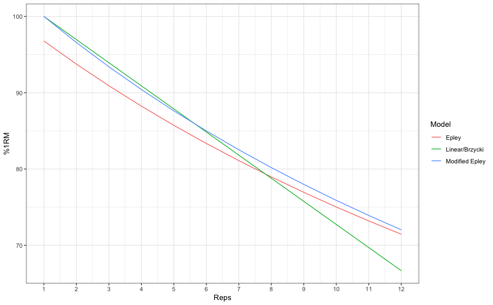
Reps-Max functions help you map out the relationship between
reps-to-failure and %1RM. Luckily, not all sets are taken to the point
of failure. {STMr} package allows you to adjust
the %1RM or repetitions using four different methods: (1) Deducted
Intensity (DI), (2) Relative Intensity (Rel Int), (3) Reps-In-Reserve
(RIR), and (4) Percentage of Maximum Reps (%MR). This is done using the
adj_ family of functions, which apply adjustments to
selected Reps-Max function/relationship.
Adjustment method is the main element of the progression table and
represents the method for progression (see [Progression] section).
Although the adjustment of the %1RM used for the target reps
(adj_perc_1RM_ family of functions) is the most common, you
can also adjust the reps for target %1RM (adj_reps_ family
of functions). Default Reps-Max function used across adjustment
functions is the max_perc_1RM_epley(). User is allowed to
provide other Reps-Max function as well as custom model parameter value.
This is extremely useful in creating individualized progression tables
and set and rep schemes.
Here is how you can use the adjustment functions to adjust %1RM when doing 5 repetitions:
# Use 10 perc deducted intensity
adj_perc_1RM_DI(5, adjustment = -0.1)
#> [1] 0.757

# Use 90 perc  relative intensity
adj_perc_1RM_rel_int(5, adjustment = 0.9)
#> [1] 0.772

# Use 2 reps in reserve
adj_perc_1RM_RIR(5, adjustment = 2)
#> [1] 0.811

# Use 70 perc max reps
adj_perc_1RM_perc_MR(5, adjustment = 0.7)
#> [1] 0.808
In addition to using adjustment, user can use multiplication
factor (mfactor parameter). This is useful for
creating ballistic, as well as conservative schemes.
In Strength
Training Manual I have suggested using factor of 2 for ballistic
exercises and using factor of 3 for control exercises
(implementing holds or various tempos of execution).
# Use ballistic adjustment (this implies doing half of the max reps possible)
# In other words, if I am doing 5 reps, I will use 10RM
adj_perc_1RM_DI(5, mfactor = 2)
#> [1] 0.75
# Use conservative adjustment (this implies doing 1/3 of the max reps possible)
# In other words, if I am doing 5 reps, I will use 15RM
adj_perc_1RM_DI(5, mfactor = 3)
#> [1] 0.667Using the RIR method, I will show you how you can customize adjustments using different Reps-Max function and custom model parameter value:
# Use Linear model
adj_perc_1RM_RIR(5, max_perc_1RM_func = max_perc_1RM_linear, adjustment = 2)
#> [1] 0.818

# Use Modifed Epley's equation with a custom parameter values
adj_perc_1RM_RIR(
  5,
  max_perc_1RM_func = max_perc_1RM_modified_epley,
  adjustment = 2,
  kmod = 0.06
)
#> [1] 0.735
Although I will show you simpler solution to this (see [Progression] section), here is how you can create simple RIR adjustment table:
# install.packages("knitr", dependencies = TRUE)
library(knitr)

at <- expand_grid(Reps = 1:5, RIR = 0:4) %>%
  mutate(
    `%1RM` = adj_perc_1RM_RIR(
      reps = Reps,
      adjustment = RIR,
      max_perc_1RM_func = max_perc_1RM_linear,
      klin = 36
    ),
    `%1RM` = round(100 * `%1RM`, 0),
    RIR = paste0(RIR, "RIR")
  ) %>%
  pivot_wider(names_from = RIR, values_from = `%1RM`)

kable(at)| Reps | 0RIR | 1RIR | 2RIR | 3RIR | 4RIR |
|---|---|---|---|---|---|
| 1 | 100 | 97 | 94 | 92 | 89 |
| 2 | 97 | 94 | 92 | 89 | 86 |
| 3 | 94 | 92 | 89 | 86 | 83 |
| 4 | 92 | 89 | 86 | 83 | 81 |
| 5 | 89 | 86 | 83 | 81 | 78 |
As you noticed, adjustment functions utilize Reps-Max function as
parameter and forwards custom model parameter value to it (or default if
custom not provided). Wrapper functions simplify this process.
{STMr} package implements two wrapper functions:
get_perc_1RM() and get_reps():
get_perc_1RM(5, method = "RelInt", model = "linear", adjustment = 0.8)
#> [1] 0.703

get_perc_1RM(5, method = "%MR", model = "linear", adjustment = 0.8, klin = 36)
#> [1] 0.854

get_reps(0.85, method = "RIR", model = "modified epley", adjustment = 2, kmod = 0.035)
#> [1] 4.04
Progressions (or progression tables) represent implemented adjustments in a systematic and organized manner across progression steps and scheme volume types (intensive, normal, and extensive). Please refer to Strength Training Manual book and Load-Exertion Tables And Their Use For Planning article series for more information about progression tables.
{STMr} package has multiple progressions implemented and
they all start with progression_. Progression functions
also allow user to utilize different Reps-Max function (default is
max_perc_1RM_epley()) and provide custom model parameter
value. This modular and flexible feature allows for easier generation of
individualized progression tables, as well as set and rep schemes.
Here is an example using Constant RIR Increment Progression using 5 repetitions and -3, -2, -1, and 0 progression steps using “normal” volume. Please note that progression steps move backwards from the Reps-Max relationship, indicated as step 0.
progression_RIR(5, step = c(-3, -2, -1, 0), volume = "normal")
#> $adjustment
#> [1] 4 3 2 1
#>
#> $perc_1RM
#> [1] 0.769 0.790 0.811 0.833
The output of progression_ functions is a
list with two elements: (1) adjustment, and
(2) perc_1RM. You can use this directly, but
progression_ function is most often used within
scheme_ functions (see Set
and Rep Schemes section).
Easier way to create progression table across different types
(grinding, ballistic, and conservative), volumes, rep ranges, and
progression steps is to use generate_progression_table()
function:
pt <- generate_progression_table(progression_RIR, type = "conservative")

head(pt)
#>           type    volume reps step adjustment perc_1RM
#> 1 conservative intensive    1   -3          3    0.714
#> 2 conservative    normal    1   -3          4    0.667
#> 3 conservative extensive    1   -3          5    0.625
#> 4 conservative intensive    2   -3          3    0.667
#> 5 conservative    normal    2   -3          4    0.625
#> 6 conservative extensive    2   -3          5    0.588
Even better approach would be to plot progression table:
plot_progression_table(progression_RIR, reps = 1:12, signif_digits = 2, type = "grinding")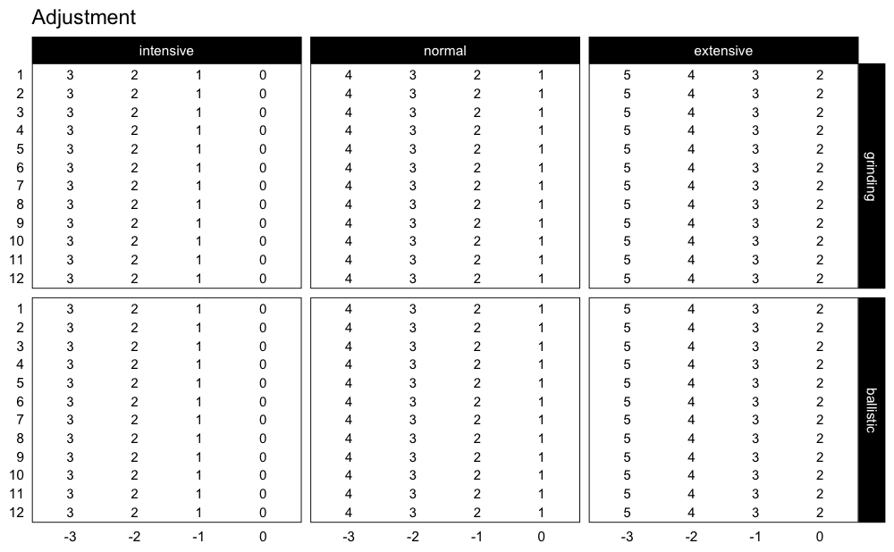
If you are interested in plotting the adjustments used, use:
plot_progression_table(progression_RIR, reps = 1:12, plot = "adjustment", type = "grinding")
progression_RIR() allows you to use custom progression
increments as well as volume increments:
plot_progression_table(
  progression_RIR,
  plot = "adjustment",
  reps = 1:12,
  step_increment = 1,
  volume_increment = 2,
  type = "grinding"
)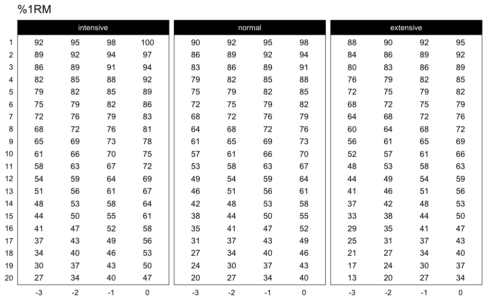
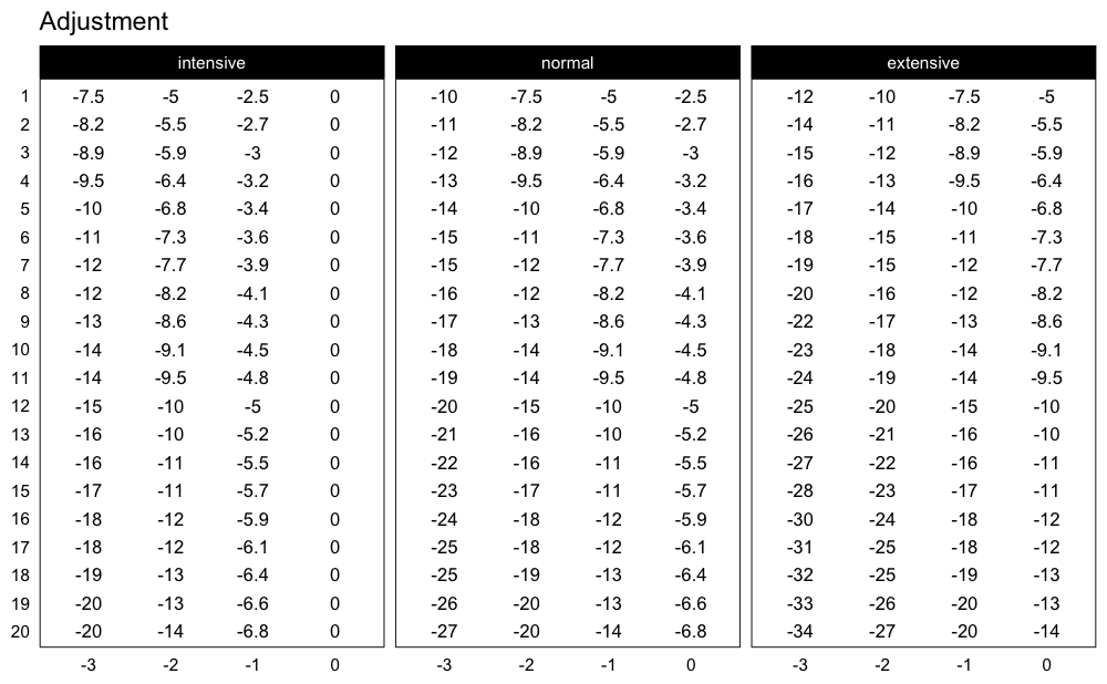
Here is another example using Perc Drop progression table and Linear/Brzycki’s model:
plot_progression_table(
  progression_perc_drop,
  max_perc_1RM_func = max_perc_1RM_linear,
  klin = 36,
  type = "grinding",
  reps = 1:20,
  signif_digits = 2
)
Here are the adjustments used in the Perc Drop progression table (deducted %1RM):
plot_progression_table(
  progression_perc_drop,
  plot = "adjustment",
  multiplier = 100,
  max_perc_1RM_func = max_perc_1RM_linear,
  klin = 36,
  type = "grinding",
  reps = 1:20,
  signif_digits = 2
)
Another useful feature implemented in {STMr} package is
a create_example() function to quickly generate strength
training program example. I will use
progression_perc_MR_variable() in this example:
example <- create_example(progression_perc_MR_variable, reps = c(5, 10), type = "grinding")

kable(example)| type | reps | volume | Step 1 | Step 2 | Step 3 | Step 4 | Step 2-1 Diff | Step 3-2 Diff | Step 4-3 Diff |
|---|---|---|---|---|---|---|---|---|---|
| grinding | 5 | intensive | 79.3 | 82.0 | 84.1 | 85.7 | 2.72 | 2.09 | 1.66 |
| grinding | 5 | normal | 72.4 | 76.3 | 79.3 | 81.6 | 3.93 | 2.95 | 2.30 |
| grinding | 5 | extensive | 58.7 | 66.9 | 72.4 | 76.3 | 8.22 | 5.49 | 3.93 |
| grinding | 10 | intensive | 67.2 | 70.3 | 72.9 | 75.0 | 3.10 | 2.57 | 2.16 |
| grinding | 10 | normal | 59.1 | 63.6 | 67.2 | 70.1 | 4.47 | 3.59 | 2.94 |
| grinding | 10 | extensive | 45.8 | 53.4 | 59.1 | 63.6 | 7.58 | 5.72 | 4.47 |
{STMr} package have the following progression tables
implemented: progression_DI(),
progression_perc_drop(),
progression_perc_MR(),
progression_perc_MR_variable(),
progression_rel_int(), progression_RIR(),
progression_RIR_increment(),
progression_variable_DI(), and
progression_variable_RIR(). You can use aforementioned
functions to explore these progression tables, and build your own.
Please refer to Load-Exertion
Tables And Their Use For Planning article series for more
information about these progression tables.
Vertical Planning represents another layer in building set and rep
schemes and it revolves around changes or progressions across time. This
involves changes to repetitions, progression steps, number of sets and
so forth. Please refer to Strength
Training Manual book for thorough information about the Vertical
Planning. Vertical Planning functions in {STMr} package
begin with vertical_.
Here is an example involving constant variant of Vertical Planning:
vertical_constant(reps = c(5, 5, 5))
#>    index step set set_id reps
#> 1      1   -3   1      1    5
#> 2      1   -3   2      2    5
#> 3      1   -3   3      3    5
#> 4      2   -2   1      1    5
#> 5      2   -2   2      2    5
#> 6      2   -2   3      3    5
#> 7      3   -1   1      1    5
#> 8      3   -1   2      2    5
#> 9      3   -1   3      3    5
#> 10     4    0   1      1    5
#> 11     4    0   2      2    5
#> 12     4    0   3      3    5
As can be seen from the code output, this Vertical Planning involves keeping the constant repetitions and decreasing progression steps. Let’s use linear Vertical Planning:
vertical_linear(reps = c(10, 10, 10), reps_change = c(0, -2, -4))
#>   index step set set_id reps
#> 1     1   -2   1      1   10
#> 2     1   -2   2      2   10
#> 3     1   -2   3      3   10
#> 4     2   -1   1      1    8
#> 5     2   -1   2      2    8
#> 6     2   -1   3      3    8
#> 7     3    0   1      1    6
#> 8     3    0   2      2    6
#> 9     3    0   3      3    6
You can also plot the vertical plan function, using
plot_vertical(). Might be easier to comprehend the
variations in different vertical plans.
plot_vertical(vertical_linear, reps = c(10, 10, 10))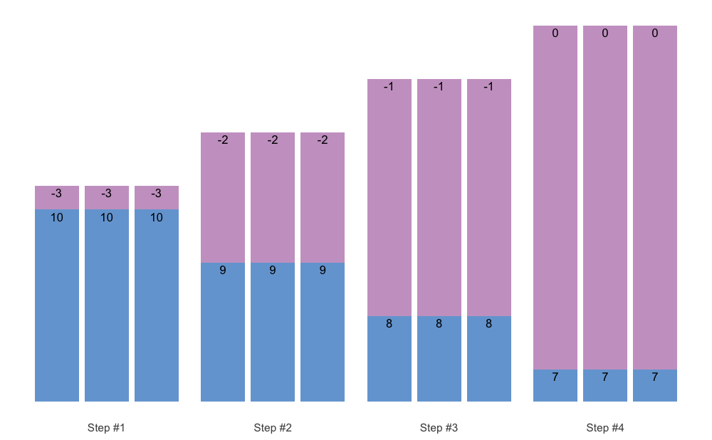
Most of these Vertical Planning functionalities can be achieved with
the generic Vertical Planning function
vertical_planning(). As can be seen from the output, result
of the Vertical Planning functions is a simple data.frame
with five columns: (1) index, (2) step, and
(3) set, (4) set_id, and reps.
Usability of Vertical Planning functions is mostly visible at the next
layer of prescription: schemes (see Set and Rep Schemes section).
{STMr} currently features the following Vertical
Planning functions: vertical_planning(),
vertical_constant(), vertical_linear(),
vertical_linear_reverse(), vertical_block(),
vertical_block_variant(),
vertical_block_undulating(),
vertical_rep_accumulation(),
vertical_set_accumulation(),
vertical_set_accumulation_reverse(),
vertical_undulating(),
vertical_undulating_reverse(),
vertical_volume_intensity().
Note: Please note that
vertical_rep_accumulation() when used with Set and Rep Schemes will yield
wrong results. I will address how to deal with this issue in Rep Accumulation section.
Set and rep schemes are the highest layer in {STMr}
package, since they utilize Reps-Max model, adjustment method,
progression table, and vertical planning. {STMr} package is
built to follow this modular approach, which makes is
extensible and flexible.
Set and rep schemes are implemented using the functions that begin
with scheme_. Here is an example for the Wave Set and Rep
Scheme (for more information about various set and rep schemes please
refer to Strength
Training Manual book):
# Wave set and rep scheme
scheme <- scheme_wave(
  reps = c(10, 8, 6, 10, 8, 6),
  # Adjusting sets to use lower %1RM (RIR Inc method used, so RIR adjusted)
  adjustment = c(4, 2, 0, 6, 4, 2),
  vertical_planning = vertical_linear,
  vertical_planning_control = list(reps_change = c(0, -2, -4)),
  progression_table = progression_RIR_increment,
  progression_table_control = list(volume = "extensive")
)

head(scheme)
#>   index step set reps adjustment perc_1RM
#> 1     1   -2   1   10      12.91    0.567
#> 2     1   -2   2    8       9.82    0.628
#> 3     1   -2   3    6       6.73    0.702
#> 4     1   -2   4   10      14.91    0.547
#> 5     1   -2   5    8      11.82    0.602
#> 6     1   -2   6    6       8.73    0.671
The output of the scheme_ functions is a simple
data.frame with the following six columns: (1)
index, (2) step, (3) set, (4)
reps, (5) adjustment, and (6)
perc_1RM.
Set and rep scheme functions offers you the ability to utilize
different vertical planning (using the vertical_planning
argument, as well as vertical_planning_control to forward
extra parameters to the vertical planning function), progression table
(using the progression_table argument, as well as
progression_table_control to forward extra parameters,
including Reps-Max function), and extra adjustments to the reps
utilized. Please note that the adjustment utilized depends on the
progression table selected (i.e., if using RIR Increment, adjustment
will be RIR). Also, the adjustment in the results is the
total adjustment, which is the sum of the progression table
adjustment and user-provided extra adjustment using the
adjustment argument. Plotting the scheme is a better way to
comprehend it:
plot(scheme)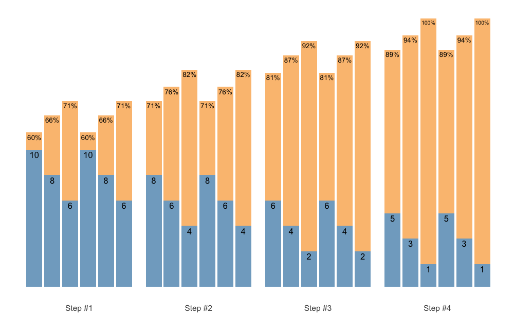
Check the Scheme plotting tips section for more information and tips on plotting schemes.
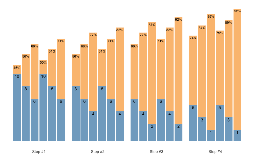
In the next example I will utilize different progression table and progression steps, as well as Linear/Brzycki’s Reps-Max model with a custom model parameter value:
# Wave set and rep scheme
scheme <- scheme_wave(
  reps = c(10, 8, 6, 10, 8, 6),
  # Since the default Wave Loading adjustments assume RIR progression table,
  # we need to set it to zero
  adjustment = 0,
  vertical_planning = vertical_planning, # Generic function
  vertical_planning_control = list(reps_change = c(0, -2, -4, -5), step = c(-6, -4, -2, 0)),
  progression_table = progression_DI,
  progression_table_control = list(
    volume = "intensive",
    max_perc_1RM_func = max_perc_1RM_linear,
    klin = 36
  )
)

plot(scheme)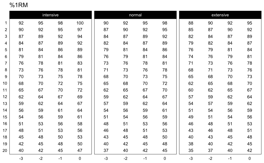
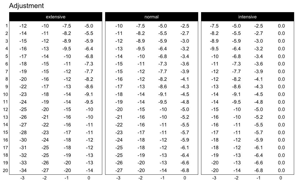
This scheme would be pretty impossible to do, since I am using the intensive variant of the Deducted Intensity progression, but in this case I have 3 heavy sets. Here is the Deducted Intensity progression table (with -2.5% decrement across volume types and progression steps):
plot_progression_table(
  progression_DI,
  max_perc_1RM_func = max_perc_1RM_linear,
  klin = 36,
  type = "grinding",
  reps = 1:20,
  signif_digits = 2
)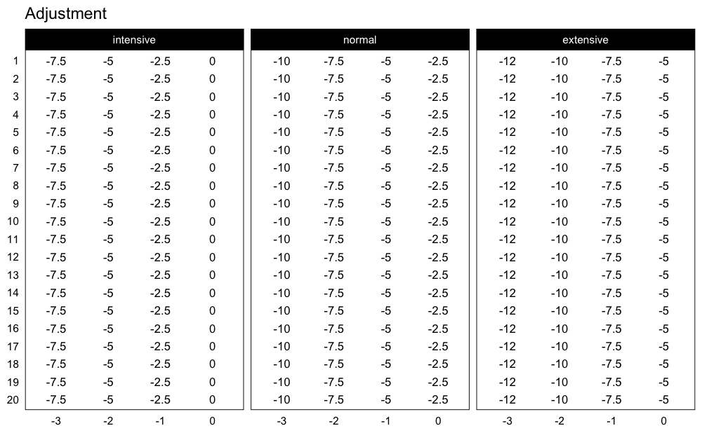
plot_progression_table(
  progression_DI,
  plot = "adjustment",
  multiplier = 100,
  max_perc_1RM_func = max_perc_1RM_linear,
  klin = 36,
  type = "grinding",
  reps = 1:20,
  signif_digits = 2
)
To make the Waves Loading scheme in the above example doable, I can apply additional adjustments to make sets easier. Since I am using Deducted Intensity, adjustments will be in %1RM:
# Wave set and rep scheme
scheme <- scheme_wave(
  reps = c(10, 8, 6, 10, 8, 6),
  adjustment = c(-15, -10, -5, -10, -5, 0) / 100,
  vertical_planning = vertical_planning, # Generic function
  vertical_planning_control = list(reps_change = c(0, -2, -4, -5), step = c(-6, -4, -2, 0)),
  progression_table = progression_DI,
  progression_table_control = list(
    volume = "intensive",
    max_perc_1RM_func = max_perc_1RM_linear,
    klin = 36
  )
)

plot(scheme)
The scheme_ functions afford you great flexibility in
designing set and rep schemes. The following set and rep schemes are
implemented in {STMr} package:
scheme_generic(), scheme_wave(),
scheme_plateau(), scheme_step(),
scheme_step_reverse(),
scheme_wave_descending(),
scheme_light_heavy(), scheme_pyramid(),
scheme_pyramid_reverse(), scheme_rep_acc(),
scheme_manual(), and scheme_perc_1RM().
+ operator{STMr} package allows you very modular approach in
designing set and rep schemes. For example, we might want to use simple
warm-up, followed with single wave, and finished with 3 sets of 5
across. To do this, we can simple add them up using the +
operator. I will explain the scheme_perc_1RM() function in
Manual scheme section.
warmup <- scheme_perc_1RM(
  reps = c(5, 5, 5),
  perc_1RM = c(0.4, 0.5, 0.6)
)

wave <- scheme_wave(vertical_planning = vertical_linear)
plateau <- scheme_plateau()

# Simply add them up
my_scheme <- warmup + wave + plateau

plot(my_scheme)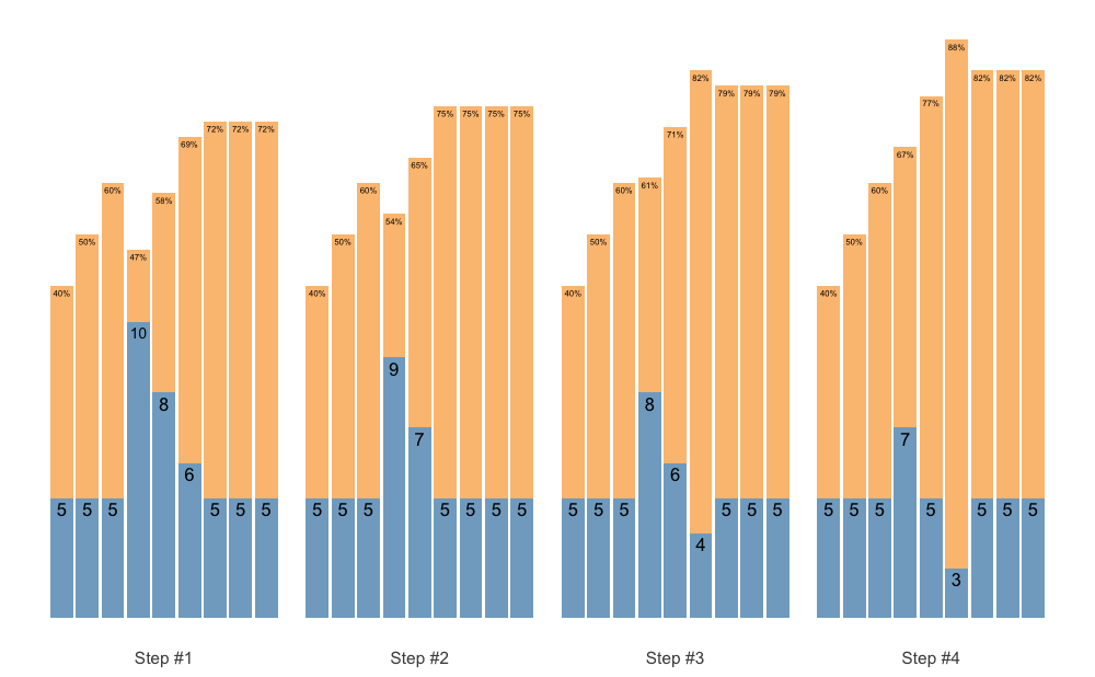
If you intend to use vertical_rep_accumulation() withing
scheme_ functions, it will yield wrong result. Here is an
example:
scheme_plateau(reps = c(5, 5, 5), vertical_planning = vertical_rep_accumulation)
#>    index step set reps adjustment perc_1RM
#> 1      1    0   1    2    -0.0273    0.910
#> 2      1    0   2    2    -0.0273    0.910
#> 3      1    0   3    2    -0.0273    0.910
#> 4      2    0   1    3    -0.0295    0.880
#> 5      2    0   2    3    -0.0295    0.880
#> 6      2    0   3    3    -0.0295    0.880
#> 7      3    0   1    4    -0.0318    0.851
#> 8      3    0   2    4    -0.0318    0.851
#> 9      3    0   3    4    -0.0318    0.851
#> 10     4    0   1    5    -0.0341    0.823
#> 11     4    0   2    5    -0.0341    0.823
#> 12     4    0   3    5    -0.0341    0.823
You need to check the perc_1RM column - it needs to be
the same across progression steps, but it is not.
This is due to the modular design of the {shorts}
package. One way to sort this out, is to use the
scheme_rep_acc() function:
scheme_rep_acc(reps = c(5, 5, 5))
#>    index step set reps adjustment perc_1RM
#> 1      1    0   1    2    -0.0341    0.823
#> 2      1    0   2    2    -0.0341    0.823
#> 3      1    0   3    2    -0.0341    0.823
#> 4      2    0   1    3    -0.0341    0.823
#> 5      2    0   2    3    -0.0341    0.823
#> 6      2    0   3    3    -0.0341    0.823
#> 7      3    0   1    4    -0.0341    0.823
#> 8      3    0   2    4    -0.0341    0.823
#> 9      3    0   3    4    -0.0341    0.823
#> 10     4    0   1    5    -0.0341    0.823
#> 11     4    0   2    5    -0.0341    0.823
#> 12     4    0   3    5    -0.0341    0.823
With some extra arguments, we can generate waves, pyramid and other schemes:
scheme_rep_acc(reps = c(10, 8, 6), adjustment = c(-0.1, -0.05, 0))
#>    index step set reps adjustment perc_1RM
#> 1      1    0   1    7    -0.1455    0.605
#> 2      1    0   2    5    -0.0909    0.699
#> 3      1    0   3    3    -0.0364    0.797
#> 4      2    0   1    8    -0.1455    0.605
#> 5      2    0   2    6    -0.0909    0.699
#> 6      2    0   3    4    -0.0364    0.797
#> 7      3    0   1    9    -0.1455    0.605
#> 8      3    0   2    7    -0.0909    0.699
#> 9      3    0   3    5    -0.0364    0.797
#> 10     4    0   1   10    -0.1455    0.605
#> 11     4    0   2    8    -0.0909    0.699
#> 12     4    0   3    6    -0.0364    0.797
Unfortunately, this will not work for the ladders and
volume-intensity scheme. The more universal approach would be
to apply rep accumulation AFTER the scheme is generated. For
this reason these is .vertical_rep_accumulation.post()
function, which works across all schemes. Just make sure to use
vertical_constant when generating the scheme (this is
default option):
scheme_ladder() %>%
  .vertical_rep_accumulation.post()
#>    index step set reps adjustment perc_1RM
#> 2      1    0   2    2         NA    0.705
#> 3      1    0   3    7         NA    0.705
#> 4      2    0   1    1         NA    0.705
#> 5      2    0   2    3         NA    0.705
#> 6      2    0   3    8         NA    0.705
#> 7      3    0   1    2         NA    0.705
#> 8      3    0   2    4         NA    0.705
#> 9      3    0   3    9         NA    0.705
#> 10     4    0   1    3         NA    0.705
#> 11     4    0   2    5         NA    0.705
#> 12     4    0   3   10         NA    0.705
scheme <- scheme_wave() %>%
.vertical_rep_accumulation.post()
plot(scheme)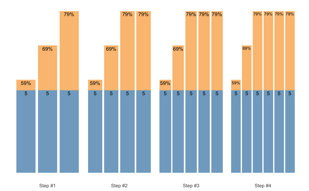
By default, .vertical_rep_accumulation.post() function
will use the highest progression step in the scheme.
Set Accumulation can happen in multiple ways. We can accumulate the last set, which is the simplest and default approach:
scheme <- scheme_step(
  reps = c(5, 5, 5),
  vertical_planning = vertical_set_accumulation
)

plot(scheme)
We can also accumulate the whole sequence, for example when using the Waves:
scheme <- scheme_wave(
  reps = c(10, 8, 6),
  vertical_planning = vertical_set_accumulation,
  vertical_planning_control = list(accumulate_set = 1:3)
)

plot(scheme)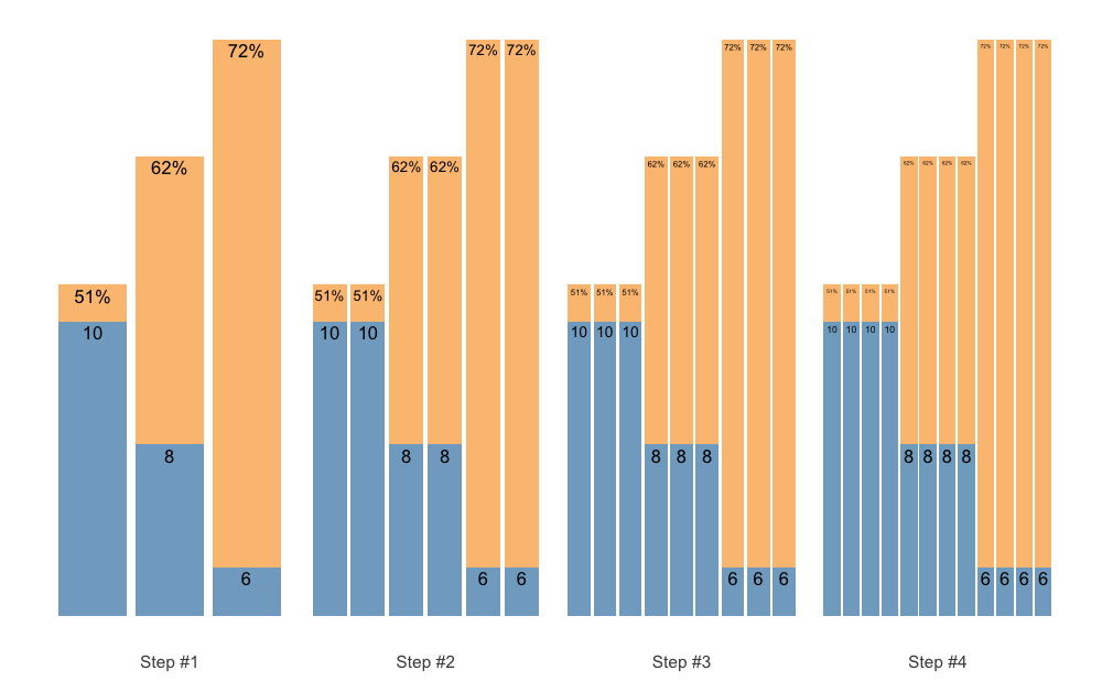
Or, instead of accumulating sequence, we can accumulate individual sets:
scheme <- scheme_wave(
  reps = c(10, 8, 6),
  vertical_planning = vertical_set_accumulation,
  vertical_planning_control = list(accumulate_set = 1:3, sequence = FALSE)
)

plot(scheme)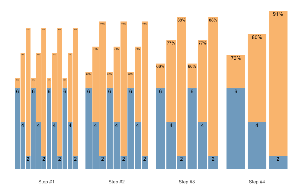
Set accumulation function is very flexible. As an another example, we
can use vertical_set_accumulation_reverse() to create a
neat accumulation-intensification progression:
scheme <- scheme_wave(
  reps = c(6, 4, 2),
  vertical_planning = vertical_set_accumulation_reverse,
  vertical_planning_control = list(accumulate_set = 1:3)
)

plot(scheme)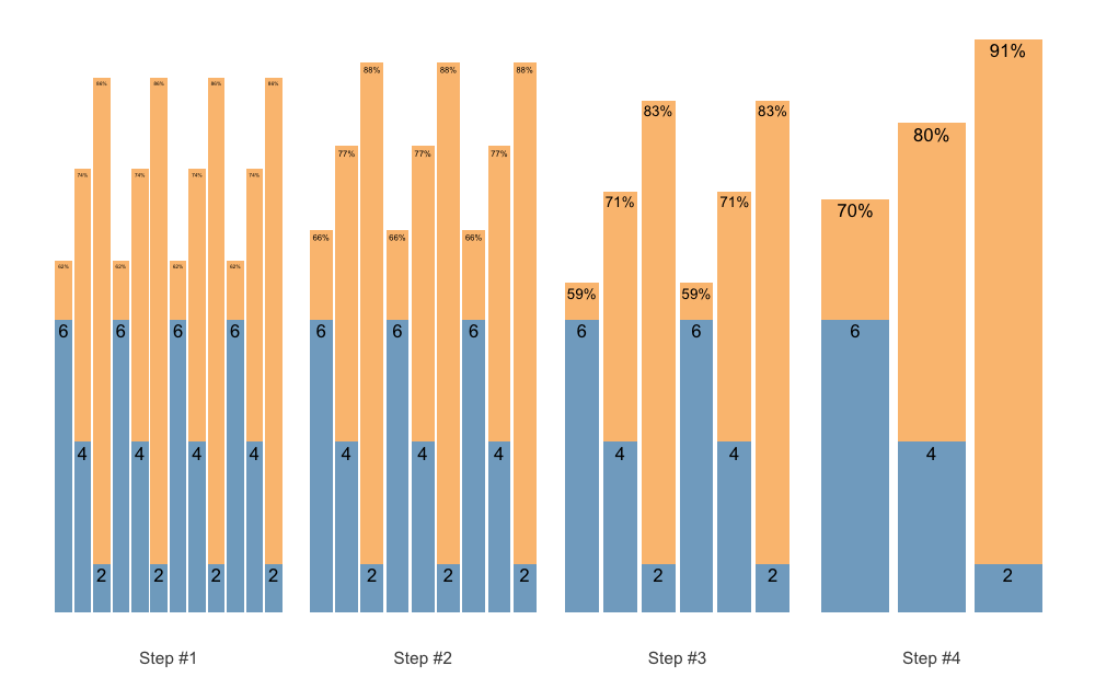
Maybe we want another progression steps:
scheme <- scheme_wave(
  reps = c(6, 4, 2),
  vertical_planning = vertical_set_accumulation_reverse,
  vertical_planning_control = list(
    accumulate_set = 1:3,
    # Lets create non-linear (aka unduating step changes)
    step = c(-2, -1, -3, 0)
  )
)

plot(scheme)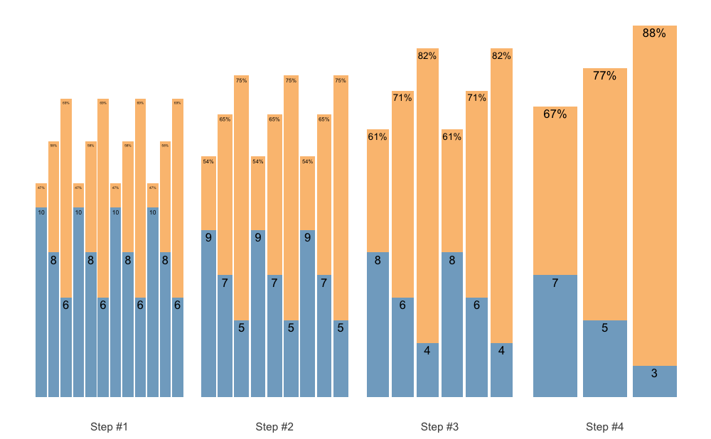
But maybe we want the reps to fall down as well, to have a even
bigger accumulation-intensification effect. In that case we case use
reps_change argument:
scheme <- scheme_wave(
  reps = c(10, 8, 6),
  vertical_planning = vertical_set_accumulation_reverse,
  vertical_planning_control = list(
    accumulate_set = 1:3,
    reps_change = c(0, -1, -2, -3)
  )
)

plot(scheme)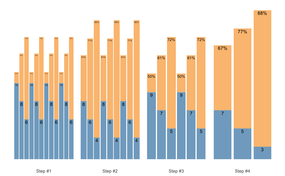
As an last example, let us create Block Undulating with reverse set accumulation:
scheme <- scheme_wave(
  reps = c(10, 8, 6),
  vertical_planning = vertical_set_accumulation_reverse,
  vertical_planning_control = list(
    accumulate_set = 1:3,
    step = c(-2, -1, -3, 0),
    reps_change = c(0, -2, -1, -3)
  )
)

plot(scheme)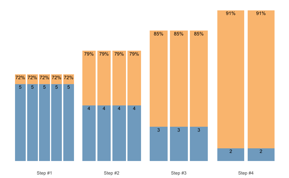
If you are looking for a pen-ultimate flexibility, then the
scheme_manual() function is there for you. It allows you to
manually code the index, step, number of sets, reps, and adjustments,
and thus provide the greatest flexibility. Here are few examples to get
you started:
scheme_df <- data.frame(
  index = 1, # Use this just as an example
  step = c(-3, -2, -1, 0),
  # Sets are just an easy way to repeat reps and adjustment
  sets = c(5, 4, 3, 2),
  reps = c(5, 4, 3, 2),
  adjustment = 0
)

# Step index is estimated to be sequences of steps
# If you want specific indexes, use it as an argument (see next example)
scheme <- scheme_manual(
  step = scheme_df$step,
  sets = scheme_df$sets,
  reps = scheme_df$reps,
  adjustment = scheme_df$adjustment
)

plot(scheme)
# Here we are going to provide our own index
scheme <- scheme_manual(
  index = scheme_df$index,
  step = scheme_df$step,
  sets = scheme_df$sets,
  reps = scheme_df$reps,
  adjustment = scheme_df$adjustment
)

plot(scheme)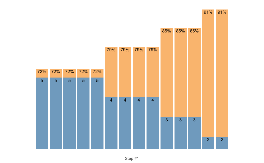
# More complicated example
scheme_df <- data.frame(
  step = c(-3, -3, -3, -3, -2, -2, -2, -1, -1, 0),
  sets = 1,
  reps = c(5, 5, 5, 5, 3, 2, 1, 2, 1, 1),
  adjustment = c(0, -0.05, -0.1, -0.15, -0.1, -0.05, 0, -0.1, 0, 0)
)

scheme_df
#>    step sets reps adjustment
#> 1    -3    1    5       0.00
#> 2    -3    1    5      -0.05
#> 3    -3    1    5      -0.10
#> 4    -3    1    5      -0.15
#> 5    -2    1    3      -0.10
#> 6    -2    1    2      -0.05
#> 7    -2    1    1       0.00
#> 8    -1    1    2      -0.10
#> 9    -1    1    1       0.00
#> 10    0    1    1       0.00

scheme <- scheme_manual(
  step = scheme_df$step,
  sets = scheme_df$sets,
  reps = scheme_df$reps,
  adjustment = scheme_df$adjustment,

  # Select another progression table
  progression_table = progression_DI,
  # Extra parameters for the progression table
  progression_table_control = list(
    volume = "extensive",
    type = "ballistic",
    max_perc_1RM_func = max_perc_1RM_linear,
    klin = 36
  )
)

plot(scheme)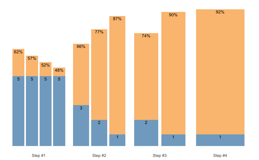
The scheme_manual() function allows you to manually
enter 1RM percentage (rather than them being calculated using
progression table):
# Provide %1RM manually
scheme_df <- data.frame(
  index = rep(c(1, 2, 3, 4), each = 3),
  reps = rep(c(5, 5, 5), 4),
  perc_1RM = rep(c(0.4, 0.5, 0.6), 4)
)

warmup_scheme <- scheme_manual(
  index = scheme_df$index,
  reps = scheme_df$reps,
  perc_1RM = scheme_df$perc_1RM
)

plot(warmup_scheme)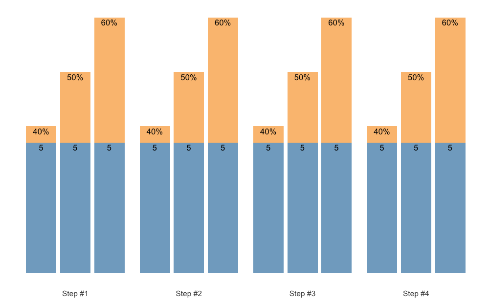
Easier method to create pre-filled 1RM percentages is to use
scheme_perc_1RM() function:
warmup_scheme <- scheme_perc_1RM(
  reps = c(5, 5, 5),
  perc_1RM = c(0.4, 0.5, 0.6),
  n_steps = 4
)

plot(warmup_scheme)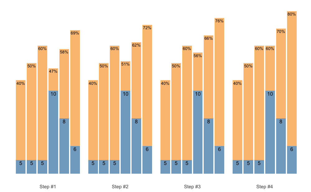
We can then use the + operator to mold the warm-up to
selected scheme. Here is an example:
plot(warmup_scheme + scheme_wave())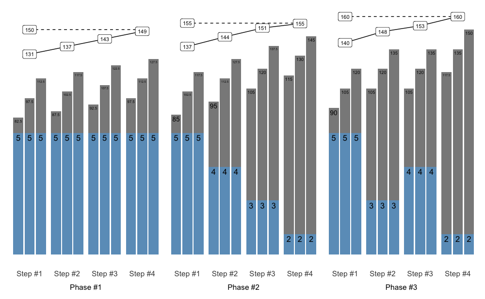
To mold multiple schemes (i.e., blocks or phases) together, use
release() function and accompanying S3 plot()
method. The release() function allows you to inspect how
multiple back-to-back schemes merge together and provide long-term
progressive overload.
To calculate weight from scheme percentages, use
prescription_1RM, which is adjusted/updated every phases
using additive_1RM_adjustment and
multiplicative_1RM_adjustment arguments. Additionally,
load_1RM is calculated using selected reps-max function.
This is done by dividing the weight used by estimated %1RM from done
repetitions. This helps in visualizing how loading trends over time.
Please check Further information
section for more info.
scheme1 <- scheme_step(vertical_planning = vertical_constant)
scheme2 <- scheme_step(vertical_planning = vertical_linear)
scheme3 <- scheme_step(vertical_planning = vertical_undulating)

release_df <- release(
  scheme1, scheme2, scheme3,
  prescription_1RM = 150,
  additive_1RM_adjustment = 5,
  multiplicative_1RM_adjustment = 1, # no adjustment
  rounding = 2.5, # round weight to the closest 2.5
  max_perc_1RM_func = max_perc_1RM_epley
)

plot(release_df)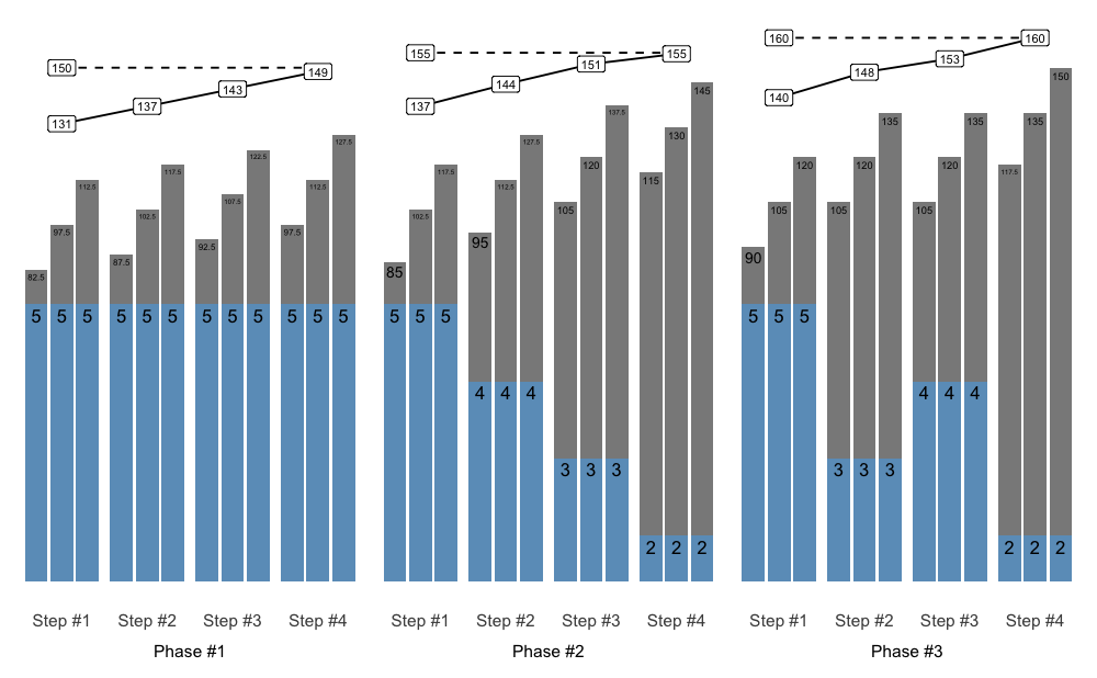
{STMr} package offers very flexible and customizable
approach to percent-based strength prescription. As explained in the
previous examples, one can use three models of Reps-Max relationship (or
write additional implementation) and apply custom model parameter values
(i.e., k, kmod, and klin for
Epley’s, Modified Epley’s, and Linear/Brzycki’s models respectively). In
addition to providing custom model parameter values, {STMr}
package offers function to estimate these parameter values.
Before introducing the estimate_ family of functions,
let’s introduce built-in datasets that we are going to use. The first
dataset is the RTF testing:
data(RTF_testing)

head(RTF_testing)
#> # A tibble: 6 × 7
#>   Athlete   `1RM` `Target %1RM` `Target Weight` `Real Weight` `Real %1RM`   nRM
#>   <chr>     <dbl>         <dbl>           <dbl>         <dbl>       <dbl> <dbl>
#> 1 Athlete A   100           0.9            90            90         0.9       6
#> 2 Athlete A   100           0.8            80            80         0.8      13
#> 3 Athlete A   100           0.7            70            70         0.7      22
#> 4 Athlete B    95           0.9            85.5          85         0.895     3
#> 5 Athlete B    95           0.8            76            75         0.789     8
#> 6 Athlete B    95           0.7            66.5          67.5       0.711    12
This dataset contains reps-to-failure tests for 12 athletes, their 1RMs and RTF sets using 90, 80, and 70% 1RM.
The next dataset is strength training log:
data(strength_training_log)

head(strength_training_log)
#> # A tibble: 6 × 8
#>   phase  week   day session     set weight  reps  eRIR
#>   <int> <int> <dbl> <chr>     <int>  <dbl> <dbl> <dbl>
#> 1     1     1     1 Session A     1   57.5    12    NA
#> 2     1     1     1 Session A     2   62.5    10     5
#> 3     1     1     1 Session A     3   70       8     3
#> 4     1     1     1 Session A     4   55      12    NA
#> 5     1     1     1 Session A     5   60      10    NA
#> 6     1     1     1 Session A     6   65       8     4
This dataset contains strength training log for a single athlete and single exercise performed in the training program. Strength training program involves doing two strength training sessions, over 12 week (4 phases of 3 weeks each). Session A involves linear wave-loading pattern starting with 2x12/10/8 reps and reaching 2x8/6/4 reps. Session B involves constant wave-loading pattern using 2x3/2/1. This dataset contains weight being used, as well as estimated/perceived reps-in-reserve (eRIR), which represent subjective rating of the proximity to failure.
{STMr} package has three types of estimation functions:
(1) simple estimation functions, (2) mixed-effect estimation functions,
and (3) quantile estimation functions. Each of these three types of
estimation functions allow you to work with (1) %1RM and repetitions to
estimate single parameter (i.e., k, kmod, or
klin parameters for Epley’s, Modified Epley’s, and
Linear/Brzycki’s models respectively), and (2) absolute weight and
repetitions, which in addition to estimating model parameter value
estimates 1RM. This represent novel technique in sports science, yet to
be validated (paper preparation currently ongoing). In the next section
I will walk you through each of these, but for more information please
refer to Load-Exertion
Tables And Their Use For Planning article series.
To demonstrate simple profile estimation I will use
RTF_testing dataset. The figure below depicts maximum
number of repetitions performed against both absolute (or raw) and
relative weights (using %1RM).
# install.packages("patchwork", dependencies = TRUE)
library(patchwork)

gg_absolute <- ggplot(RTF_testing, aes(x = `Real Weight`, y = nRM, color = Athlete)) +
  theme_bw() +
  geom_point(alpha = 0.8) +
  geom_line(alpha = 0.8) +
  xlab("Weight (kg)") +
  theme(legend.position = "none")

gg_relative <- ggplot(RTF_testing, aes(x = `Real %1RM` * 100, y = nRM, color = Athlete)) +
  theme_bw() +
  geom_point(alpha = 0.8) +
  geom_line(alpha = 0.8) +
  xlab("%1RM") +
  ylab(NULL)

gg_absolute + gg_relative + plot_layout(widths = c(1, 1.1))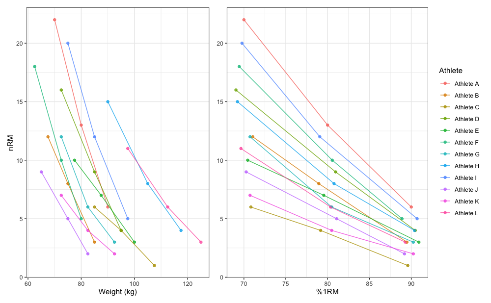
Let’s use Athlete B from RTF testing dataset to estimate individual model parameter values for Epley’s, Modified Epley’s, and Linear/Brzycki’s models.
athlete_rtf <- RTF_testing %>%
  filter(Athlete == "Athlete B")

# Estimate Epley's model
m1 <- estimate_k(
  perc_1RM = athlete_rtf$`Real %1RM`,
  reps = athlete_rtf$nRM
)

coef(m1)
#>     k
#> 0.034

# Estimate Modifed Epley's model
m2 <- estimate_kmod(
  perc_1RM = athlete_rtf$`Real %1RM`,
  reps = athlete_rtf$nRM
)

coef(m2)
#>   kmod
#> 0.0381

# Estimate Linear/Brzycki's model
m3 <- estimate_klin(
  perc_1RM = athlete_rtf$`Real %1RM`,
  reps = athlete_rtf$nRM
)

coef(m3)
#> klin
#>   35
These simple estimation functions return the nls object,
since nls() function is used to estimate model parameter
values. You can also use the ... feature of the simple
estimation function to forward extra arguments to nls()
function.
Estimate functions also allow you to use reverse statistical
model (using reverse = TRUE argument), where predictor is
number of reps (i.e., nRM), and target variable is %1RM.
Estimate functions offer various observation weighting options.
Options are ‘none’, ‘reps’, ‘load’, ‘eRIR’, ‘reps x load’, ‘reps x
eRIR’, ‘load x eRIR’, and ‘reps x load x eRIR’ and are set using the
weighted = argument.
Novel technique implemented into {STMr} is estimation of
both 1RM and model parameter value from absolute weights, rather than
from %1RM for which you need known 1RM:
# Estimate Epley's model
m1 <- estimate_k_1RM(
  weight = athlete_rtf$`Real Weight`,
  reps = athlete_rtf$nRM
)

coef(m1)
#>       k     0RM
#>  0.0316 93.3874

# Since Epley's model estimated 0RM and NOT 1RM, use
# the following function to get 1RM
get_predicted_1RM_from_k_model(m1)
#> [1] 90.5

# Estimate Modifed Epley's model
m2 <- estimate_kmod_1RM(
  weight = athlete_rtf$`Real Weight`,
  reps = athlete_rtf$nRM
)

coef(m2)
#>    kmod     1RM
#>  0.0307 90.5246

# Estimate Linear/Brzycki's model
m3 <- estimate_klin_1RM(
  weight = athlete_rtf$`Real Weight`,
  reps = athlete_rtf$nRM
)

coef(m3)
#> klin  1RM
#> 45.6 88.8
This novel technique allows for embedded testing (please
refer to Strength
Training Manual and Load-Exertion
Tables And Their Use For Planning article series for more
information) using the strength training log data. In the case where
sets are not taken to failure, one can also utilize subjective rating of
perceived/estimated RIR (eRIR argument). This technique
will be applied to log analysis in the Quantile estimation section.
The simple estimation function allow for the estimation for a single individual. Simple estimation can also be used for pooled analysis (i.e., all athletes and/or exercises pooled together) with %1RM to get the generic or average model parameter value. Unfortunately, this will not work with the absolute weights as predictors, hence the need to normalize the predictors using relative weight or %1RM.
Here is an example of pooled profile estimation using the
RTF_testing dataset and Modified Epley’s model:
m_pooled <- estimate_kmod(
  perc_1RM = RTF_testing$`Real %1RM`,
  reps = RTF_testing$nRM,
  # Use weighting
  weighted = "reps x load"
)

coef(m_pooled)
#>   kmod
#> 0.0449

pred_df <- data.frame(perc_1RM = seq(0.65, 1, length.out = 100)) %>%
  mutate(nRM = max_reps_modified_epley(perc_1RM = perc_1RM, kmod = coef(m_pooled)))

ggplot(RTF_testing, aes(x = `Real %1RM` * 100, y = nRM)) +
  theme_bw() +
  geom_point(aes(color = Athlete), alpha = 0.8) +
  geom_line(aes(color = Athlete), alpha = 0.8) +
  xlab("%1RM") +
  geom_line(data = pred_df, aes(x = perc_1RM * 100, y = nRM), size = 1.5, alpha = 0.8)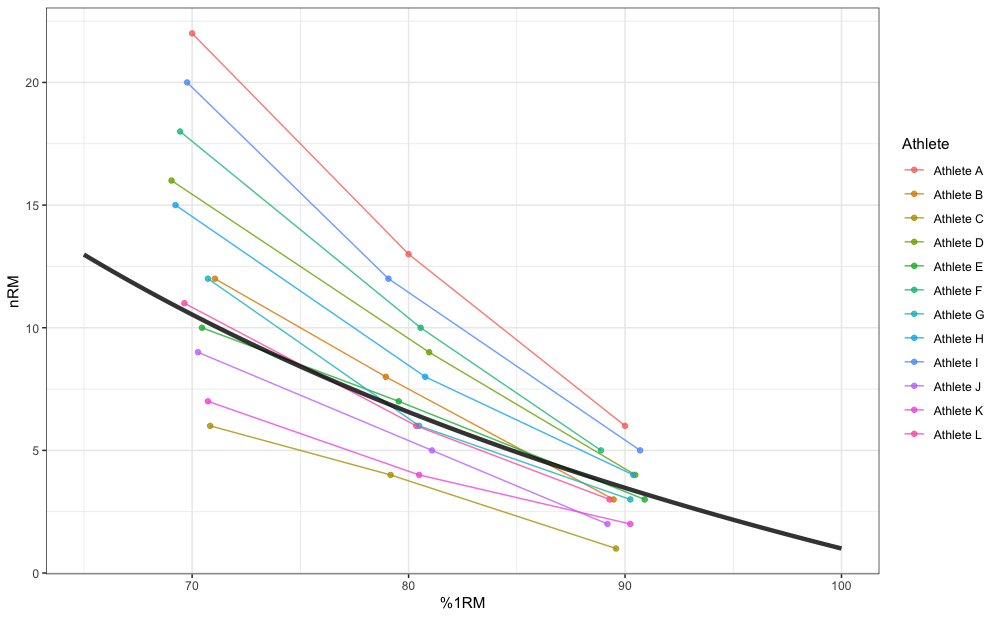
When analyzing multiple individuals, particularly when absolute
weights are used instead of %1RM, one needs to utilize mixed-effect
approach. {STMr} package implements non-linear mixed-effect
model using the nlme() function from the
{nlme} package. Mixed-effects estimation functions in
{STMr} package end with _mixed. You can also
use the ... feature of the mixed-effects estimation
functions to forward extra arguments to nlme()
function.
Here is how to perform mixed-effects model using Modified Epley’s model and %1RM as predictor:
mm1 <- estimate_kmod_mixed(
  athlete = RTF_testing$Athlete,
  perc_1RM = RTF_testing$`Real %1RM`,
  reps = RTF_testing$nRM
)

summary(mm1)
#> Nonlinear mixed-effects model fit by maximum likelihood
#>   Model: nRM ~ ((kmod - 1) * perc_1RM + 1)/(kmod * perc_1RM)
#>   Data: df
#>   AIC BIC logLik
#>   131 136  -62.7
#>
#> Random effects:
#>  Formula: kmod ~ 1 | athlete
#>           kmod Residual
#> StdDev: 0.0178    0.658
#>
#> Fixed effects:  kmod ~ 1
#>       Value Std.Error DF t-value p-value
#> kmod 0.0422   0.00529 24    7.97       0
#>
#> Standardized Within-Group Residuals:
#>    Min     Q1    Med     Q3    Max
#> -2.222 -0.769 -0.322  0.263  1.167
#>
#> Number of Observations: 36
#> Number of Groups: 12

coef(mm1)
#>             kmod
#> Athlete A 0.0206
#> Athlete B 0.0382
#> Athlete C 0.0796
#> Athlete D 0.0300
#> Athlete E 0.0456
#> Athlete F 0.0264
#> Athlete G 0.0404
#> Athlete H 0.0324
#> Athlete I 0.0233
#> Athlete J 0.0552
#> Athlete K 0.0692
#> Athlete L 0.0453
Please note the difference between fixed parameter value of
kmod estimated using the mixed-effects model (equal to
0.042) and our previous pooled model (equal to 0.045).
In addition to estimating fixed parameter value, mixed-effects model also estimates random parameter values (i.e., individual athlete model parameter values). Mixed-effects model can be thought as a combination of pooled model (i.e., fixed effects) and multiple individual models (i.e., random effects). Figure below depicts random effects (i.e., individual predictions), fixed effects (i.e., group predictions; thick line), as well as pooled simple model predictions (dashed thick line):
pred_rnd_df <- expand_grid(
  athlete = unique(RTF_testing$Athlete),
  perc_1RM = seq(0.65, 1, length.out = 100)
) %>%
  mutate(nRM = predict(mm1, newdata = data.frame(athlete = athlete, perc_1RM = perc_1RM)))

pred_fix_df <- data.frame(perc_1RM = seq(0.65, 1, length.out = 100)) %>%
  mutate(nRM = max_reps_modified_epley(perc_1RM = perc_1RM, kmod = summary(mm1)$coefficients$fixed))

gg <- ggplot(RTF_testing, aes(x = `Real %1RM` * 100, y = nRM)) +
  theme_bw() +
  geom_point(aes(color = Athlete), alpha = 0.8) +
  geom_line(data = pred_rnd_df, aes(x = perc_1RM * 100, y = nRM, color = athlete), alpha = 0.8) +
  geom_line(data = pred_fix_df, aes(x = perc_1RM * 100, y = nRM), alpha = 0.8, size = 1.5) +
  geom_line(data = pred_df, aes(x = perc_1RM * 100, y = nRM), size = 1.5, alpha = 0.8, linetype = "dashed") +
  xlab("%1RM")
gg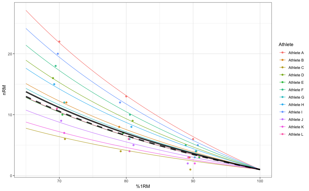
{STMr} package also implements mixed-effect models that
utilize absolute weight values. As alluded previously, this is novel
technique that besides estimating Reps-Max profile, also estimates 1RM.
Here is how to perform mixed-effects Linear/Brzycki’s model using
absolute weights:
mm2 <- estimate_klin_1RM_mixed(
  athlete = RTF_testing$Athlete,
  weight = RTF_testing$`Real Weight`,
  reps = RTF_testing$nRM
)

summary(mm2)
#> Nonlinear mixed-effects model fit by maximum likelihood
#>   Model: nRM ~ (1 - (weight/oneRM)) * klin + 1
#>   Data: df
#>   AIC BIC logLik
#>   180 189    -84
#>
#> Random effects:
#>  Formula: list(klin ~ 1, oneRM ~ 1)
#>  Level: athlete
#>  Structure: General positive-definite, Log-Cholesky parametrization
#>          StdDev Corr
#> klin     15.809 klin
#> oneRM    13.544 -0.145
#> Residual  0.632
#>
#> Fixed effects:  klin + oneRM ~ 1
#>       Value Std.Error DF t-value p-value
#> klin   46.2      4.82 23     9.6       0
#> oneRM 101.5      4.06 23    25.0       0
#>  Correlation:
#>       klin
#> oneRM -0.163
#>
#> Standardized Within-Group Residuals:
#>    Min     Q1    Med     Q3    Max
#> -1.601 -0.238  0.103  0.388  0.988
#>
#> Number of Observations: 36
#> Number of Groups: 12

coef(mm2)
#>           klin oneRM
#> Athlete A 75.2  96.2
#> Athlete B 45.4  88.9
#> Athlete C 25.3 107.1
#> Athlete D 53.3 100.5
#> Athlete E 33.9 106.1
#> Athlete F 62.5  85.3
#> Athlete G 43.2  95.8
#> Athlete H 50.2 123.8
#> Athlete I 67.2 103.2
#> Athlete J 34.4  85.0
#> Athlete K 24.8  95.5
#> Athlete L 39.4 130.1
Here is how this looks graphically:
pred_rnd_df <- expand_grid(
  athlete = unique(RTF_testing$Athlete),
  weight = seq(
    min(RTF_testing$`Real Weight`) * 0.9,
    max(RTF_testing$`Real Weight`) * 1.1,
    length.out = 100
  )
) %>%
  mutate(nRM = predict(mm2, newdata = data.frame(athlete = athlete, weight = weight))) %>%
  filter(nRM >= 1)


gg <- ggplot(RTF_testing, aes(x = `Real Weight`, y = nRM)) +
  theme_bw() +
  geom_point(aes(color = Athlete), alpha = 0.8) +
  geom_line(data = pred_rnd_df, aes(x = weight, y = nRM, color = athlete), alpha = 0.8) +
  xlab("Weight (kg)")
gg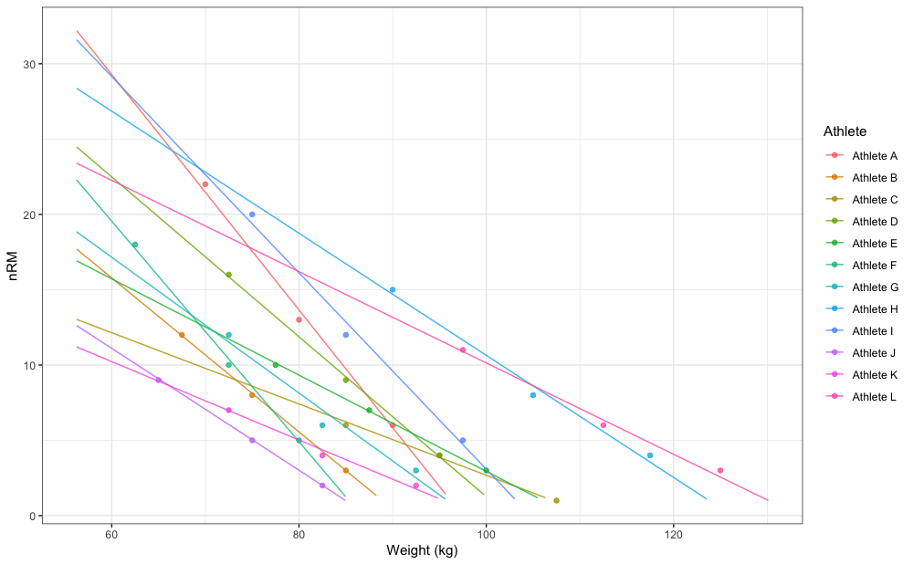
Mixed-effects functions implemented in {STMr} package
allows you to set-up random parameters using random=
function argument. In the previous example both 1RM and
klin parameters are treated as random, but you can make
klin fixed:
mm3 <- estimate_klin_1RM_mixed(
  athlete = RTF_testing$Athlete,
  weight = RTF_testing$`Real Weight`,
  reps = RTF_testing$nRM,
  random = oneRM ~ 1
)

summary(mm3)
#> Nonlinear mixed-effects model fit by maximum likelihood
#>   Model: nRM ~ (1 - (weight/oneRM)) * klin + 1
#>   Data: df
#>   AIC BIC logLik
#>   199 205  -95.4
#>
#> Random effects:
#>  Formula: oneRM ~ 1 | athlete
#>         oneRM Residual
#> StdDev:  13.3     2.05
#>
#> Fixed effects:  klin + oneRM ~ 1
#>       Value Std.Error DF t-value p-value
#> klin   47.6      3.44 23    13.8       0
#> oneRM 101.6      4.23 23    24.0       0
#>  Correlation:
#>       klin
#> oneRM -0.293
#>
#> Standardized Within-Group Residuals:
#>    Min     Q1    Med     Q3    Max
#> -1.497 -0.315 -0.110  0.500  2.120
#>
#> Number of Observations: 36
#> Number of Groups: 12

coef(mm3)
#>           klin oneRM
#> Athlete A 47.6 107.6
#> Athlete B 47.6  88.7
#> Athlete C 47.6 102.0
#> Athlete D 47.6 102.6
#> Athlete E 47.6 100.7
#> Athlete F 47.6  90.8
#> Athlete G 47.6  94.8
#> Athlete H 47.6 123.5
#> Athlete I 47.6 111.2
#> Athlete J 47.6  82.4
#> Athlete K 47.6  89.6
#> Athlete L 47.6 125.4
It is easier to grasp this graphically:
pred_rnd_df <- expand_grid(
  athlete = unique(RTF_testing$Athlete),
  weight = seq(
    min(RTF_testing$`Real Weight`) * 0.9,
    max(RTF_testing$`Real Weight`) * 1.1,
    length.out = 100
  )
) %>%
  mutate(nRM = predict(mm3, newdata = data.frame(athlete = athlete, weight = weight))) %>%
  filter(nRM >= 1)


gg <- ggplot(RTF_testing, aes(x = `Real Weight`, y = nRM)) +
  theme_bw() +
  geom_point(aes(color = Athlete), alpha = 0.8) +
  geom_line(data = pred_rnd_df, aes(x = weight, y = nRM, color = athlete), alpha = 0.8) +
  xlab("Weight (kg)")
gg
In my opinion this doesn’t make much sense. If you are interested in
estimating group or generic klin (or
k or kmod) model parameter values, use fixed
estimates, but allow it to vary (i.e. to be random effect). Estimated
fixed klin value from random 1RM and random
klin model is equal to 46.24, where with the above fixed
klin and random 1RM it is equal to 47.62. Regardless of
your statistical modeling preference, {STMr} package allows
you implementation of each.
So far we have estimated Reps-Max profiles using sets to failure. This approach demands designated testing session(s). But what if we could estimate Reps-Max profiles as well as 1RMs from training log data? This would allow “embedded” testing, since we would not need designated testing sessions or sets, but we could use normal training log data.
When sets are not taken to failure, one way to estimate max reps that can be performed is to utilize subjective rating of perceived reps-in-reserve (pRIR or eRIR). For example, if I perform 100kg for 5 reps on the bench press and I rate it with 2pRIR, I can assume that is 7RM load (i.e., 5 reps + 2pRIR).
strength_training_log dataset contains both reps
performed as well as eRIR values, including weight used. High eRIR
values (>5eRIR) are treated as missing-data (i.e., unreliable). Here
is the pooled plot from 12 weeks of training log data for a single
exercise:
gg <- ggplot(strength_training_log) +
  theme_bw() +
  geom_jitter(
    aes(x = weight, y = reps + eRIR),
    size = 2,
    shape = 1,
    width = 0.2,
    height = 0.2,
    alpha = 0.8
  ) +
  xlab("Weight (kg)")

gg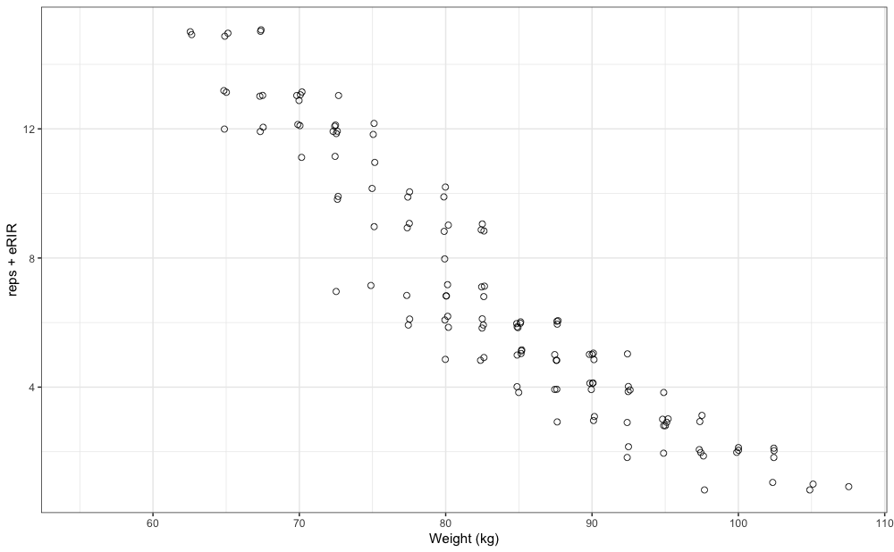
We are interested in finding both the “best” and “worst” profiles (as
well as estimated 1RMs). To achieve this, we will utilize quantile
non-linear regression. This quantile non-linear estimation is
implemented in {STMr} package using the nlrq()
function from the {quantreg} package. Quantile estimation
functions ends with _quantile. You can also use the
... feature of the quantile estimation functions to forward
extra arguments to nlrq() function.
For the “best” performance profile we can use 0.9 quantile, and for “worst” we can use 0.1 quantile. I will utilize Linear/Brzycki’s model. For more information please refer to Load-Exertion Tables And Their Use For Planning article series.
mq_best <- estimate_klin_1RM_quantile(
  weight = strength_training_log$weight,
  reps = strength_training_log$reps,
  eRIR = strength_training_log$eRIR,
  tau = 0.9
)

summary(mq_best)
#>
#> Call: quantreg::nlrq(formula = nRM ~ (1 - (weight/`1RM`)) * klin +
#>     1, data = df, start = list(klin = 1, `1RM` = max(df$weight)),
#>     tau = tau, control = list(maxiter = 10000, k = 2, InitialStepSize = 0,
#>         big = 1e+20, eps = 1e-07, beta = 0.97), trace = FALSE)
#>
#> tau: [1] 0.9
#>
#> Coefficients:
#>      Value  Std. Error t value Pr(>|t|)
#> klin  36.88   1.48      24.91    0.00
#> 1RM  105.36   1.15      91.97    0.00
coef(mq_best)
#>  klin   1RM
#>  36.9 105.4

mq_worst <- estimate_klin_1RM_quantile(
  weight = strength_training_log$weight,
  reps = strength_training_log$reps,
  eRIR = strength_training_log$eRIR,
  tau = 0.1
)

summary(mq_worst)
#>
#> Call: quantreg::nlrq(formula = nRM ~ (1 - (weight/`1RM`)) * klin +
#>     1, data = df, start = list(klin = 1, `1RM` = max(df$weight)),
#>     tau = tau, control = list(maxiter = 10000, k = 2, InitialStepSize = 0,
#>         big = 1e+20, eps = 1e-07, beta = 0.97), trace = FALSE)
#>
#> tau: [1] 0.1
#>
#> Coefficients:
#>      Value Std. Error t value Pr(>|t|)
#> klin 26.00  3.90       6.67    0.00
#> 1RM  97.50  1.89      51.71    0.00
coef(mq_worst)
#> klin  1RM
#> 26.0 97.5
Graphically, these profiles look like this:
pred_df_best <- tibble(weight = seq(60, 120, length.out = 100)) %>%
  mutate(nRM = predict(mq_best, newdata = data.frame(weight = weight))) %>%
  filter(nRM >= 1)

pred_df_worst <- tibble(weight = seq(60, 120, length.out = 100)) %>%
  mutate(nRM = predict(mq_worst, newdata = data.frame(weight = weight))) %>%
  filter(nRM >= 1)

gg +
  geom_line(data = pred_df_best, aes(x = weight, y = nRM)) +
  geom_line(data = pred_df_worst, aes(x = weight, y = nRM), linetype = "dashed")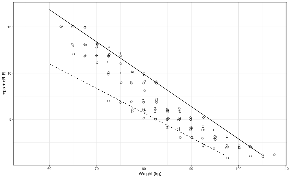
In the previous example we have used all 12 weeks of strength
training log data (i.e., pooled). We can perform the rolling
analysis using the estimate_rolling_1RM() function.
estimate_rolling_1RM() allows you to use different
functions (i.e., estimate_k_1RM(),
estimate_kmod_1RM(), estimate_klin_1RM(),
estimate_k_1RM_quantile(),
estimate_kmod_1RM_quantile(), and
estimate_klin_1RM_quantile()). Here is an example using
previous 6 days (i.e., one phase, or 3 rolling weeks):
estimate_rolling_1RM(
  weight = strength_training_log$weight,
  reps = strength_training_log$reps,
  eRIR = strength_training_log$eRIR,
  day_index = strength_training_log$day,
  window = 6,
  estimate_function = estimate_kmod_1RM_quantile,
  tau = 0.9
)
#> # A tibble: 19 × 3
#>    day_index   kmod `1RM`
#>        <int>  <dbl> <dbl>
#>  1         6 0.0404  98.8
#>  2         7 0.0368  98.5
#>  3         8 0.0400 101.
#>  4         9 0.0383 101.
#>  5        10 0.0431 104.
#>  6        11 0.0432 104.
#>  7        12 0.0455 106.
#>  8        13 0.0385 104.
#>  9        14 0.0385 104.
#> 10        15 0.0410 106.
#> 11        16 0.0415 107.
#> 12        17 0.0415 107.
#> 13        18 0.0410 106.
#> 14        19 0.0410 106.
#> 15        20 0.0415 107.
#> 16        21 0.0381 106.
#> 17        22 0.0381 106.
#> 18        23 0.0364 106.
#> 19        24 0.0382 107.
In the following example, I am using rolling 3 weeks estimation of
the “best” and “worst” 1RM, as well as the kmod parameter
using 0.1 and 0.9 quantiles:
est_profiles <- function(.x) {
  res <- estimate_rolling_1RM(
    weight = strength_training_log$weight,
    reps = strength_training_log$reps,
    eRIR = strength_training_log$eRIR,
    day_index = strength_training_log$day,
    window = 6,
    estimate_function = estimate_kmod_1RM_quantile,
    tau = .x$tau
  )

  tibble(tau = .x$tau, res)
}

data.frame(tau = c(0.1, 0.9)) %>%
  rowwise() %>%
  do(est_profiles(.)) %>%
  ungroup() %>%
  pivot_longer(cols = -c(tau, day_index), names_to = "param") %>%
  group_by(day_index, param) %>%
  summarise(lower = min(value), upper = max(value)) %>%
  ungroup() %>%
  # Plot
  ggplot(aes(x = day_index)) +
  theme_bw() +
  geom_ribbon(aes(ymin = lower, ymax = upper, fill = param), color = "black", alpha = 0.5) +
  facet_wrap(~param, scales = "free_y") +
  xlab("Day index") +
  ylab(NULL) +
  theme(legend.position = "none")
This analysis represents novel technique and the time will tell how
valid is it and how to interpret it correctly. But at least we have very
powerful, transparent, and flexible open-source tool:
{STMr} package.
Since I have developed the {STMr} package to help me
write the Strength
Training Manual Volume 3 book, the plotting functionalites are vast
and flexible. Here are the few tip you can use.
S3 plot method for plotting {STMr} schemes
allow for three different types of plots: (1) bar
(default), (2) vertical, and (3) fraction.
Here is the default bar plot:
scheme <- scheme_wave(
  reps = c(10, 8, 6),
  vertical_planning = vertical_linear
)

plot(scheme)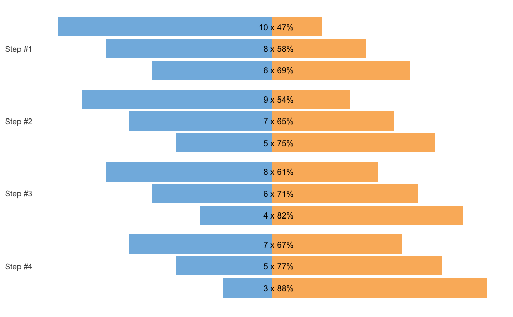
Another way to plot the scheme is using the vertical
method.
plot(scheme, type = "vertical")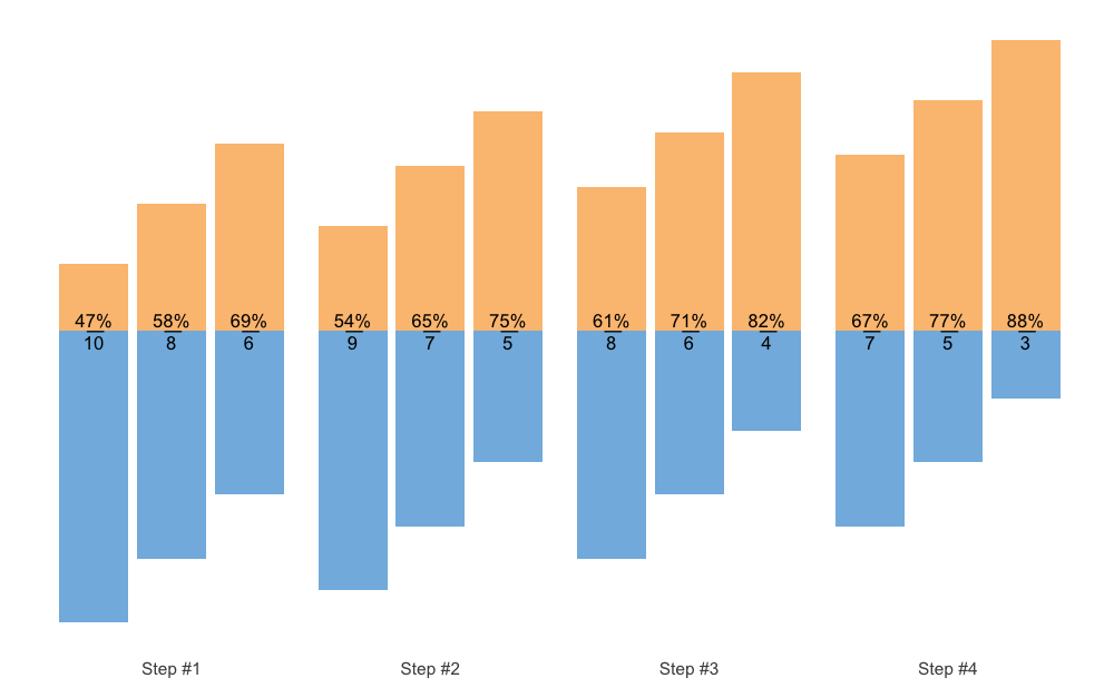
And the final method is to use fraction method, which is
very similar to the Olympic weightlifting log notation:
plot(scheme, type = "fraction")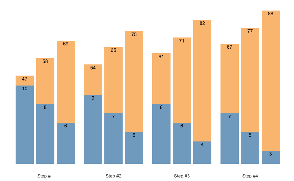
To avoid printing %, which will make %1RM
labels bigger, use perc_str = "":
plot(scheme, perc_str = "")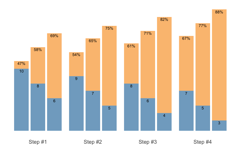
S3 plot method for plotting {STMr} schemes
allow you to set the font size. This can be useful later once we used
facets.
plot(scheme, font_size = 20)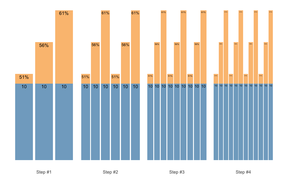
The plotting allows for the flexible labels, using the
{ggfittext} package, which fits the labels so they do not
exit the bars. Here is an example using the Set Accumulation vertical
plan:
scheme <- scheme_wave(
  reps = c(10, 10, 10),
  vertical_planning = vertical_set_accumulation,
  vertical_planning_control = list(accumulate_set = 1:3, sequence = TRUE)
)

plot(scheme)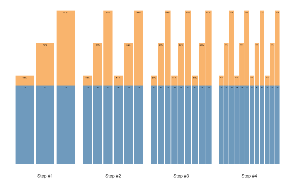
Using the size argument, you can set the maximum label
size. This is useful if you want to avoid having different sizes of
labels on your plot. The labels will still be shrinked if needed, but it
will not be bigger than selected font size:
plot(scheme, size = 5)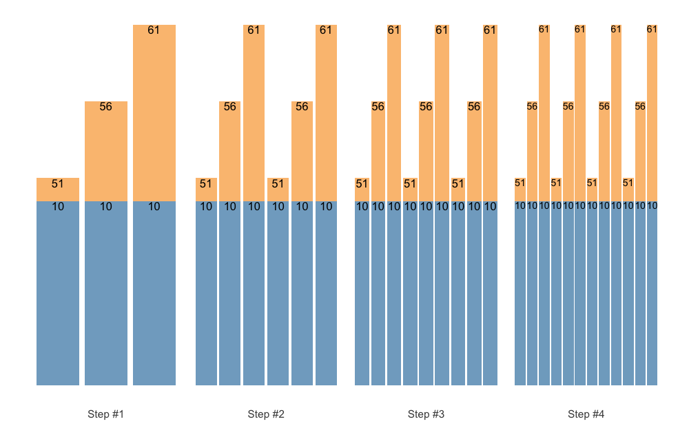
You can also set padding of the labels. Let’s remove %
and set the padding:
plot(
  scheme,
  perc_str = "",
  padding.x = grid::unit(0.2, "mm"),
  padding.y = grid::unit(0.2, "mm"),
)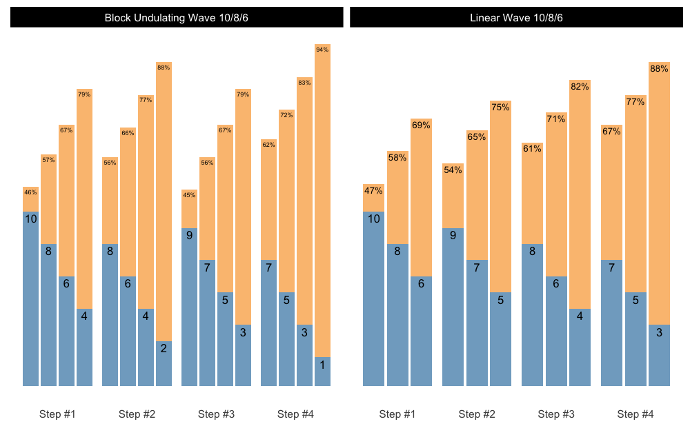
Let’s say you want to generate multiple schemes and want to plot them. Here is how you can do it easily:
scheme_1 <- scheme_wave(
  reps = c(10, 8, 6),
  vertical_planning = vertical_linear
)

scheme_2 <- scheme_wave(
  reps = c(10, 8, 6, 4),
  vertical_planning = vertical_block_undulating
)

scheme_df <- rbind(
  data.frame(scheme = "Linear Wave 10/8/6", scheme_1),
  data.frame(scheme = "Block Undulating Wave 10/8/6", scheme_2)
)

# We need to set the same class to allow for S3 plotting method
class(scheme_df) <- class(scheme_1)

# Since the plot() returns ggplot object, we can create facets
plot(scheme_df) +
  facet_wrap(~scheme)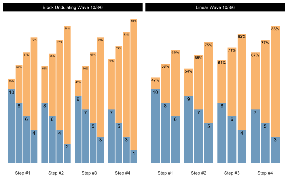
To find out more, please check the Create
Custom Set and Rep Schemes With {STMr} course, which covers a lot of
ground and the utilization of the {STMr} package in
depth.
{STMr}If you are using {STMr} package in your publications,
please use the following citation:
citation("STMr")
#> To cite package 'STMr' in publications use:
#>
#>   Jovanović M (2026). _STMr: Strength Training Manual R-Language
#>   Functions_. R package version 0.1.7,
#>   <https://github.com/mladenjovanovic/STMr>.
#>
#> A BibTeX entry for LaTeX users is
#>
#>   @Manual{STMr-package,
#>     title = {{STMr}: Strength Training Manual R-Language Functions},
#>     author = {Mladen Jovanović},
#>     year = {2026},
#>     note = {R package version 0.1.7},
#>     url = {https://github.com/mladenjovanovic/STMr},
#>   }
If you plan using estimation models in your commercial or
non-commercial products, please contact me at my email:
coach.mladen.jovanovic @ gmail.com