![]()
The RPIV package implements residual prediction tests
for the well-specification of linear instrumental variable (IV) models,
as developed in Scheidegger, Londschien and Bühlmann (2025).
For a response \(Y_i \in \mathbb R\), endogenous regressors \(X_i \in \mathbb R^p\), instruments \(Z_i \in \mathbb R^d\) with \(d \ge p\), and optional exogenous control variables \(C_i \in \mathbb R^q\), the package provides two related procedures:
RPIV_test(): a residual prediction test for the
well-specification of the linear IV model under strong
identification;weak_RPIV_test(): a weak-IV-robust version that tests
the conditional moment restriction at a given candidate parameter value
and can be inverted to obtain confidence sets.The main question addressed by the package is whether the linear IV model is an appropriate description of the data.
More formally, the standard test targets the null hypothesis \(H_0:\ \exists \beta \in \mathbb R^p \text{ such that } \mathbb E[Y_i - X_i^T\beta \mid Z_i] = 0 \quad \text{a.s.}\) which is implied by the well-specification of the linear IV model (with mean-independence assumption on the errors).
When exogenous controls are present, the model is understood as allowing for an additional linear term in \(C_i\), and in the standard implementation these controls are added both to \(X\) and to \(Z\).
The weak-IV-robust procedure instead considers, for a fixed candidate value \(\beta_0 \in \mathbb R^p\), the null hypothesis \(H_0(\beta_0):\ \exists \theta \in \mathbb R^q \text{ such that } \mathbb E[Y_i - X_i^T\beta_0 - C_i^T\theta \mid Z_i, C_i] = 0 \quad \text{a.s.}\) By fixing \(\beta_0\), the test avoids relying on strong identification. Inverting the test over a grid of candidate values yields a confidence set for the endogenous coefficient(s). If this confidence set is empty, the data provide evidence against well-specification.
The underlying idea of both tests is to check for signal in the residuals using a random forest. For a detailed discussion of the methodology, we refer to Scheidegger, Londschien and Bühlmann (2025). A Python implementation of the residual prediction approach is available in the package ivmodels.
You can install the released CRAN version of RPIV
with
install.packages("RPIV")You can install the development version from GitHub with
devtools::install_github("cyrillsch/RPIV")The following example illustrates how to test the well-specification
of a linear IV model with RPIV_test(). We simulate three
outcomes: one generated from a well-specified linear IV model, and two
generated under misspecification.
set.seed(1)
n <- 200
C <- rnorm(n)
Z <- cbind(rnorm(n), C + rnorm(n))
H <- rnorm(n)
X <- Z[, 1] - Z[, 2] + rnorm(n)

Y1 <- X - C + H + rnorm(n)
Y2 <- X - C + H + Z[, 1]^2 + rnorm(n)
Y3 <- 2 * sign(X - C) + H + rnorm(n)
We apply RPIV_test() to all three outcomes. By default,
the function uses a heteroskedasticity-robust variance estimator.
library(RPIV)

result1 <- RPIV_test(Y = Y1, X = X, C = C, Z = Z)
result2 <- RPIV_test(Y = Y2, X = X, C = C, Z = Z)
result3 <- RPIV_test(Y = Y3, X = X, C = C, Z = Z)

result1$p_value
#> [1] 0.1575286
result2$p_value
#> [1] 0.0004228503
result3$p_value
#> [1] 0.005525054
As expected, the null of well-specification is not rejected for
Y1, while it is rejected for Y2 and
Y3 at significance level \(\alpha
= 0.05\).
The function weak_RPIV_test() provides a weak-IV-robust
version of the procedure. Rather than testing whether there exists some
coefficient vector satisfying the conditional moment restriction, it
tests the null hypothesis at a fixed candidate value
beta.
A key use case is test inversion: we evaluate the test over a grid of candidate values and retain those values that are not rejected, i.e., the values that are compatible with well-specification at a given significance level. Under well-specification, the resulting set is a confidence set for the endogenous coefficient. If this set is empty, the data provide evidence against well-specification of the linear IV model.
In the next example, we consider two outcomes:
Y1, generated from a correctly specified linear IV
model with true coefficient beta = 1;Y2, generated under misspecification through an
additional nonlinear term in the instrument.set.seed(1)
n <- 200
Z <- rnorm(n)
C <- rnorm(n)
H <- rnorm(n)
X <- Z + rnorm(n) + H
Y1 <- X - C - H + rnorm(n) # correctly specified, true beta = 1
Y2 <- X - C - H + Z^2 + rnorm(n) # misspecified conditional moment restrictionWe now construct the weak-IV-robust test for both outcomes.
library(RPIV)

test_statistic1 <- weak_RPIV_test(Y = Y1, X = X, C = C, Z = Z)
test_statistic2 <- weak_RPIV_test(Y = Y2, X = X, C = C, Z = Z)
Next, we evaluate the test over a grid of candidate values. Since the
test statistic is asymptotically standard Gaussian under the null, we
obtain one-sided p-values as 1 - pnorm(statistic). The
confidence set at level 1 - alpha is then the set of
candidate values whose p-values are at least alpha.
beta_grid <- seq(-1, 3, by = 0.05)
alpha <- 0.05

stats1 <- sapply(beta_grid, function(b) test_statistic1(b, "fit"))
pvals1 <- 1 - pnorm(stats1)
confset1 <- beta_grid[pvals1 >= alpha]

stats2 <- sapply(beta_grid, function(b) test_statistic2(b, "fit"))
pvals2 <- 1 - pnorm(stats2)
confset2 <- beta_grid[pvals2 >= alpha]
The confidence sets obtained by inversion are:
confset1
#>  [1] 0.45 0.50 0.55 0.60 0.65 0.70 0.75 0.80 0.85 0.90 0.95 1.00 1.05 1.10 1.15
#> [16] 1.20 1.25 1.30 1.35 1.40 1.45 1.50 1.55 1.60 1.65 1.70
confset2
#> numeric(0)
For the correctly specified outcome Y1, the confidence
set contains values close to the true parameter beta = 1.
For the misspecified outcome Y2, the confidence set is
empty reflecting the fact that no candidate value satisfies the
conditional moment restriction.
It is also useful to visualize the p-values over the grid. Values
above the horizontal line at alpha = 0.05 belong to the
confidence set.
plot(beta_grid, pvals1,
     type = "l",
     xlab = expression(beta),
     ylab = "p-value",
     main = "Weak-IV-Robust Confidence Set by Test Inversion: Correctly Specified")
abline(h = alpha, lty = 2)
abline(v = 1, lty = 3)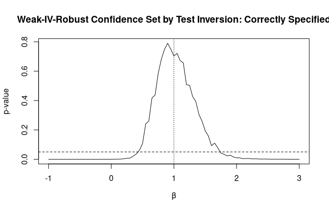
plot(beta_grid, pvals2,
     type = "l",
     xlab = expression(beta),
     ylab = "p-value",
     main = "Weak-IV-Robust Confidence Set by Test Inversion: Misspecified")
abline(h = alpha, lty = 2)
abline(v = 1, lty = 3)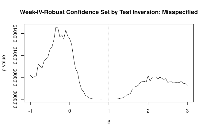
In this example we used type = "fit", which reuses the
tuning parameters obtained at the TSLS residuals and only refits the
random forest for each candidate value. This is often a good compromise
between statistical accuracy and computational cost when evaluating the
test on a grid.
Other options for the argument type are
"tune_and_fit", which retunes and refits the random forest
for the current candidate value, and "recalculate", which
reuses the partition obtained at the TSLS residuals and only recomputes
leaf means.
The package also supports cluster-robust inference. In the next example, we simulate clustered data with 50 clusters of size 4. The linear IV model is well-specified, but valid inference requires accounting for the clustering structure.
set.seed(1)
n <- 200
clustering <- rep(1:50, length.out = n)

Z <- rep(rnorm(1:50), length.out = n) + 0.1 * rnorm(n)
H <- rep(rnorm(1:50), length.out = n) + 0.1 * rnorm(n)
X <- Z + rep(rnorm(1:50), length.out = n) + 0.1 * rnorm(n)
Y <- X + H + rep(rnorm(1:50), length.out = n) + 0.1 * rnorm(n)
We apply the test with three different variance estimators: homoskedastic, heteroskedastic, and cluster-robust.
result <- RPIV_test(
  Y = Y,
  X = X,
  C = NULL,
  Z = Z,
  variance_estimator = c("homoskedastic", "heteroskedastic", "cluster"),
  clustering = clustering
)

result$homoskedastic$p_value
#> [1] 0.02844595
result$heteroskedastic$p_value
#> [1] 0.01728716
result$cluster$p_value
#> [1] 0.1347029
In this setting, only the cluster-robust variance estimator should typically avoid spurious rejection at significance level \(\alpha = 0.05\).
More examples can be found in Scheidegger, Londschien and Bühlmann (2025) and in the accompanying GitHub repository RPIV_Application.
Cyrill Scheidegger, Malte Londschien and Peter Bühlmann. Machine-learning-powered specification testing in linear instrumental variable models. Preprint, arXiv:2506.12771, 2025.